The whole essence of the VLOOKUP function in Excel (for beginners)

Of course, the VLOOKUP function is one of the most difficult for a beginner. It has a large number of arguments and no less number of possible applications. It is used especially often by advanced users, because if the range contains a huge amount of information, then manually look for the required value to display it in the formula, and then make adjustments when it changes. If you use this function, everything can be easily automated.

Syntax and features of using the VLOOKUP function

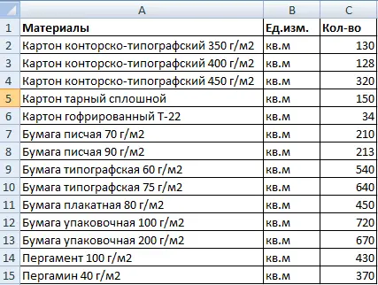
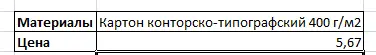
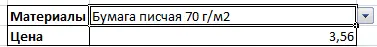
Suppose you are the manager of a warehouse that stores various materials, such as packages and containers for storing various items. And you have delivered products in a specific quantity, and it is set in Excel.

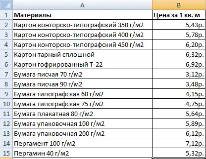
In another table, the price of each of the materials is given.

Our task is to determine how much each of the goods received at the warehouse costs. To achieve this goal, it is necessary to record in the first table the cost from the second. Then multiply one value by another. This way you can define what you want.

More precisely, the sequence of actions is as follows:

1. We bring the appearance of the table into the form we need by inserting two columns called “Price” and “Cost / Amount”. In this case, you need to apply the currency format to the cells. 
2. Click on the cell that is the first one in our “Price” column. In our case, it has the address D2. Using the function wizard, the user can always find VPR in the “References and arrays” category, regardless of the version of Excel. And there are two methods to call the function wizard. The first is to click on the fx button next to the formula input line. The second is the key combination SHIFT + F3. After the function we need is selected, we must press the OK button to confirm our actions. There is another way to call this function. You need to go to the “Formulas” tab and find the same item “References and arrays” there.
   

   

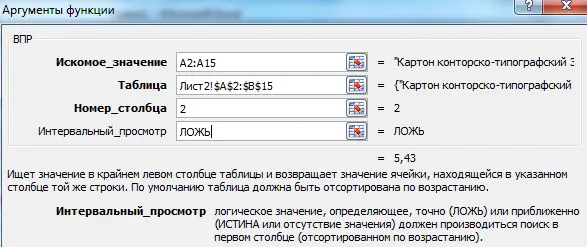
3. Next, we need to configure the function by entering our parameters into it. To do this, a special window will appear, which contains several arguments in which the user can enter their own values:
   • The desired value. In the case of our table, it is a list of product names, that is, the first column. It is this information that should be searched for in the second table.
     

     

   • Table. This is the set of cells that will be searched. In this example, this is the second table with the price list. We carry out the transition to it and select the necessary values. 
     

     

     The data must be fixed so that Excel does not change links depending on the location of the cell in which the formula is inserted. To do this, you need to make it absolute, which is easily done using the F4 key. The fact that everything worked out, we will understand by the specific dollar sign in front of the links to rows and columns.

   • Column number. In this argument, we write the number two.
   • Interval viewing. This parameter is needed if you are looking for only approximate data. This argument can take two values ​​”True” and “False”. We will write the second option, because we need accurate information.
     

     

4. After that, press the “OK” button.
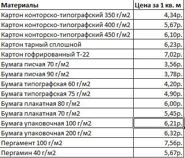
5. Further, the function is multiplied to the entire column, using the autocomplete handle, pulling the lower right corner of the cell in a downward direction. 

As a result, we get such a nice sign. The next diagram is very simple. In order to find the value of the received products in the warehouse, it is necessary to multiply the quantity of the product by its price. 

After applying the VLOOKUP function, the two tables turned out to be related. In the event of a price change, the total cost of all goods that came to the warehouse will also change. If this is the case, then everything is OK. But in some situations, you need to avoid such a problem.

How to do it? You can use Paste Special. The sequence of actions is as follows:

1. Select the desired column and right-click the mouse.
2. Copy the column.
3. We leave the selection, right-click again and click “Paste Special”, after which a menu will appear in which you need to set the radio button next to the “Values” item.

At the very end, you need to confirm your actions using the “OK” button.

Now there will be no formula in the cells, and therefore the values ​​will not change when the price of the item is adjusted.

Express comparison of two ranges

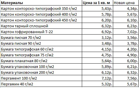
Suppose we have changed the price, and in connection with this, it is necessary to compare the old and new prices. Doing it manually is problematic. It’s good to have a function VPR.

Here is a simple guide on how to do it:

1. Create a New Price column in the old price list.
   

   

2. We click on the first cell and insert the VLOOKUP function in the way described above (via the fx button), since it is the most convenient for a beginner. As you gain professionalism, you can enter the formula manually. In our case, it will look like this. =ВПР($A$2:$A$15;’новый прайс’!$A$2:$B$15;2;ЛОЖЬ). In simple words, we need to compare the A2:A15 range in two price lists. After that, insert the new information into the old one in the “New Price” column.
   

   

Further, price information is compared manually or using Excel logical operators. You can also apply conditional formatting and highlight in red the rows where the price has changed. But this is the level of a professional. 

Using multiple conditions for a formula VPR

Up to this point, we have used only one condition – the name of the product. In practice, there are situations when you have to compare significantly more ranges according to a much larger number of criteria. In this case, you need to understand how to use multiple conditions for a function VPR.

Here is a small table to illustrate.

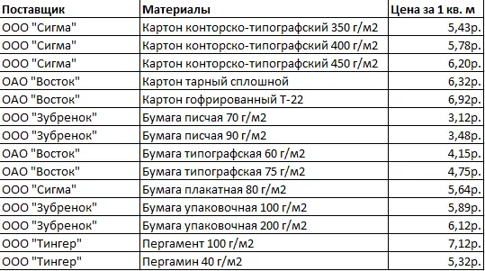
Suppose we are faced with the task of determining at what cost corrugated cardboard was imported from the manufacturer OAO Vostok. In this case, we need two conditions:

1. Материал.
2. Manufacturer.

But that’s not all, because each manufacturer imports several goods at once. How can you get out of this situation? That’s how:

1. The leftmost column is appended to the table so that vendors and materials are in the same group.
   

   

2. The criteria also need to be combined.
   

   

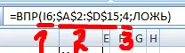
3. The cursor is placed in the desired location, and the arguments of the function are indicated in brackets (or through the appropriate dialog box). =VLOOKUP(I6,$A$2:$D$15,FALSE). Excel will then determine the required cost.
   

   

VPR and drop down list

Suppose some of the information we have is in the form of a drop-down list. In our case, this is the description of the goods. Our task is to act in such a way that after choosing the name of the product, the user has the opportunity to immediately see its cost. 

First you need to create the dropdown itself:

1. Left-click on cell E2 to select it. 
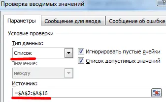
2. Move to the “Data” tab, and there find the item “Data Validation”.
   

   

3. Specify the source of information. As it we use the names of the goods. We expose the data type itself – a list.
   

   

After we click the OK button, a dropdown list will appear.

The next task is to ensure that the desired value is automatically recorded in the column with the price as soon as the user selects the desired product. To do this, you need to click on cell E9, since this is where the price is recorded in our table, and follow these instructions:

1. Click on the fx button, which will open the function wizard. This dialog box selects the function VPR.
2. As the first argument, specify the cell that contains the drop-down list. As the second – a range with the names of products and their cost. Column two. The function, as a result, takes on this form. =VLOOKUP(E8,A2:B16,FALSE)
3. After pressing the “ENTER” key, we get the desired result.
   

   

After each product correction, the price also changes.

It’s so easy to use a dropdown in combination with a function VPR. As you can see, Excel performs all actions automatically. It is enough just to figure out how this function works, and there will be a huge number of applications for it.

Why is the function not working

As you can see, using the function VPR the user is able to get almost any information from spreadsheets. However, in some cases, the user may encounter failure to use it. Why is this happening? There are many reasons for this. We will choose the most common ones.

Need an exact match

The last argument “Span” is not strictly necessary, but it is important to understand that the default value is TRUE. Therefore, for the function without this argument to work correctly, the values ​​must be sorted in ascending order.

Therefore, if a unique value is required, then it is mandatory to specify the last argument with a value of FALSE.

Fixing links to the table is required

You will probably need to apply several of these functions at once in order to get more data. If a VPR will be copied into several cells, it is important to make some of the links absolute. 

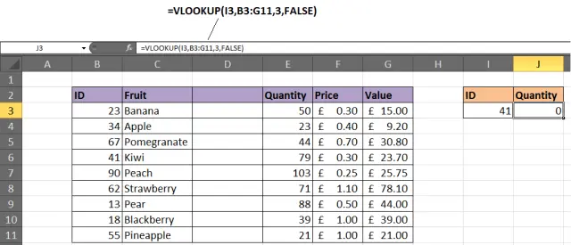
This can be seen very well in the example below. Incorrect ranges have been entered here, and because of this, the function does not want to work.

To solve this problem, simply press the F4 key to fix the link address.

In simple words, the formula should take the following form.

=VLOOKUP(($H$3,$B$3:$F$11,FALSE)

Column inserted

What is the “column number” argument for? To tell the function exactly what data should be retrieved. 

This is the problem with the fact that you need to pass a number as an argument. After all, it is enough just to insert an extra column in this place, as the performance of the formula is in question and everything needs to be redone.

But no matter how tragic this situation may seem, it has two solutions at once. If changes to the table after the final version of the document is created are not required, you can simply lock it. Then users who read the document will not be able to insert an extra column.

But this is not always the case. Then the second solution will come to the rescue. We know that another function can be used as a function argument. Here is the solution. You just need to use the function MORE EXPOSED, which returns the correct column number. 

Increasing the size of the table

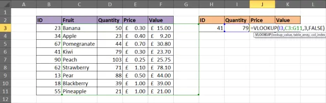
After adding new lines to the document, you may need to change the formula using the function VPRso that they are also analyzed for the presence of a particular string. This screenshot shows an example of this error. Here the formula ignores some rows of the table and therefore cannot find the desired fruit.

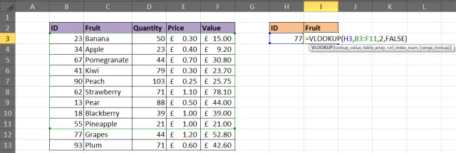
To solve this problem, you need to turn the range into a table. After that, new rows will be automatically added to the table and to the formula VPR, respectively. It is also possible to use a named range instead of a table.

The function does not know how to parse the data on the left

Yes, there is such a restriction in the function VPRand will have to put up with it. She does not know how to receive data from those columns that are located on the left. The function can only find the required values ​​in the leftmost column and to the right of it.

The solution to this problem is generally outside the plane of the function VPR. In simple terms, it does not need to be used at all. As an alternative that does not have this limitation, you can use a combination of functions INDEX и MORE EXPOSED. 

Duplicate data

Another drawback of the function is that it can only extract the first found value, you need to remove duplicates using the “Delete Duplicates” button located on the “Data” tab.

It is also possible to use a pivot table in case duplicates are needed.

Conclusions

Function VPR has a huge number of applications. And no matter how big the article is, it will still not be possible to cover everything. Therefore, you need to turn on the imagination and learn how to apply VPR along with other features for maximum results.

We see that there are enough restrictions in it too. But with the right approach, you can get out of any difficult situation.