


To find out the arithmetic average of several cells, it will not take much effort. It is enough to use the formula = HEART. But what if the weight of one of the values is greater than the rest? For example, in a large number of schools, tests or assignments may have different values. In order to make the correct calculations in such a situation, it is necessary to calculate the weighted average.
Despite the absence of this Excel function, there is another function that does most of the work for the user: =SUMPRODUCT.
This formula is very simple, and even those who have not used it before will be able to act like a professional. This weighted average method can be used in all versions of Excel and even Google Sheets.
Table setup
To calculate a weighted average, at least two columns are required. The first one (that is, column B in the example we described) is written for all assignments or tests. The second column (C in our case) describes the weighting factors. Their value directly affects the assessment for a specific task on the overall test result.
What is weight? At first glance, this is a percentage of the total. But in general, all weights correct the score set by the teacher by a certain amount upwards. It is very good that the formula we are describing corrects the estimates, regardless of what weights are added on top.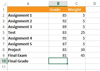
Entering a formula
Now, after our table has been set up, we paste the function into cell B10 (but you can use any empty cell you like). As with any formula, you first need to write the = sign.
First you need to enter the function =SUMPRODUCT and open parenthesis:
=SUMPRODUCT(
After that, you need to add parameters to the function. It itself can have any number of arguments, but usually two are used. In the case we are describing, the first parameter will be the range of values B2:B9, that is, the cells that are used to indicate scores for assignments and tests.
=SUMPRODUCT(B2:B9
The second parameter is the range C2;C9, covering the weight values. A comma must be used to separate all arguments. And finally, after entering the values, you must put the second bracket.
=SUMPRODUCT(B2:B9, C2:C9)
Next, the second part of the formula is added, into which to divide the value returned by the function =SUMPRODUCT. This part is the sum of all values. We’ll see later why this is so important.
So, to enter the division sign, you need to write the / sign, and then enter the function =SUM. It is enough for us to prescribe a set of weights (C2:C9) as a function parameter. It is important to close the parenthesis after that.
=СУММПРОИЗВ(B2:B9, C2:C9)/СУММ(C2:C9)
And it’s all! After pressing the “Enter” key on the keyboard, Excel will automatically determine the weighted average. In our case, the final score is 83.6.
How the formula works
Now let’s look at each part of this formula in detail to see how it functions. Let’s start with the formula SUMPRODUCT, whichmultiplies (that is, finds the derivative) each score by a weighting factor, after which it adds up all the results. Simply put, it adds up all the results of the multiplication that was carried out before. So, for the first task, she multiplies 85 by 5, and in the case of the test results – 83 by 25.
If you’re wondering why it’s necessary to multiply the values in the first place, think like this: the points for the tasks with the highest weight increase by a greater number of times. So, the second task is counted 5 times, and the final exam – 45 times. Therefore, the final exam is able to change the final score more strongly.
Compared to the standard function HEART, then the latter will enter each position into the sample only once, not paying attention to its significance.
If you want to know what calculations Excel actually does, then the calculations are done as follows:
=(B2*C2)+(B3*C3)+(B4*C4)+(B5*C5)+(B6*C6)+(B7*C7)+(B8*C8)+(B9*C9)
It’s good that you don’t need to write such a long formula where you can get confused with certain elements, because the function SUMPRODUCT does it automatically.
If this function is run by itself, then this function will give us a huge value – 10450. And this is far from the average value of all input values, adjusted for a weighting factor. And in order to understand what is the average value, it is necessary to divide the formula by the sum of all weights. Thus, the value will be 83,6.
The second part of the formula is very useful as it allows the program to automatically correct the result. It is also important to remember that the weighting factors must be greater than or equal to 100%. It can be one, 1,5, 15, 10,100. It’s just that when one or more weights are increased, the second part of the formula is automatically divided by a larger number. Therefore, the answer will still be correct, no matter what changes are made to the table. Moreover, you can reduce the weight, and still everything will work correctly. Say, cool?