Contents
Helen Bradley explains the intricacies of working with a function VPR in Microsoft Excel when searching for data in a table.
When you need to find information in a table, Excel’s search functions can help you do the job. In earlier versions of Excel, there was Substitution Wizard, with which it was easy enough to set up a search, but in Excel 2010 it is no longer there. Now, if you need a search formula, you will have to create it manually. In this article, I’ll show you how to harness the power of search functionality in Excel spreadsheets.
Basics
Microsoft Excel has several search functions, among them VLOOKUP (VLOOKUP), a very similar function HLOOKUP (GPR) and LOOKUP (VIEW). Function VPR used to look up data in a table. It searches for the value you are looking for in the first column of the table and returns the corresponding value from the other column.
When the data is arranged differently, use GPRto find the desired value in the top row of the table and return the corresponding value from the given row below. Function VIEW has two forms – vector and array, and can return a value from one column, one row or from an array (similar to VLOOKUP and HLOOKUP). Of these three functions, you will most likely use VPR much more often than others. That is what I will focus on in this article. In general, if you understand and can apply the function VPR, then you can deal with GPR.
Syntax of the VLOOKUP function
To use VPR to return a value from a table, you need to tell Excel what value to look for in the first column of the table, the range in which the table is located, and the column where the result is that the function should return.
When you specify a table range, Excel looks for the lookup value you specified in the first column of that range. As a rule, these are the row headers of your data. To specify a column number, you just need to specify its ordinal number in the given range. For example, 1 is the first column of the range, 2 is the one following him to the right, and so on. If you specify a number that is outside the specified range, for example, less than 1 or more than the number of columns in the range, you will receive an error.
This function has one more optional argument that allows you to search for an approximate or exact match of the desired value, with the first mode being used by default. If you set the exact match search mode, i.e. the last argument is FALSE (FALSE), the table may not be sorted. If you set the search mode to an inexact match, i.e. last argument is not specified or equal TRUE CODE (TRUE), you must sort the table in ascending order, otherwise the function may return an incorrect result. When searching for an inexact match, Excel looks for a value equal to the one you are looking for, and if there is none, it uses the closest one that is less than the one you are looking for.
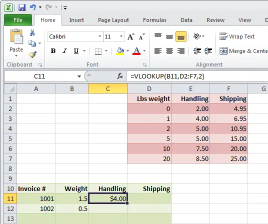
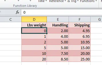
So, for example, this table shows the weight in pounds (Lbs weight), as well as the cost of handling and transportation. We can use the function VPRto find the value of the weight and determine the cost of handling (Handling) and transportation (Shipping) a consignment of goods of this weight. Of course, the weight of most batches of goods will not have the same flat values, so we use as the last argument TRUE CODE (TRUE), or do not specify it at all. In this case, our formula will find the result, even without an exact match. Do not forget to sort the table so that the data in the first column is in ascending order.
VLOOKUP in action
If we try to match the weight in 1.5 pounds, we find that there is no exact match. In this case, the function VPR will return the largest value that is not greater than the one you are looking for. Therefore, if we are looking for 1.5 and we do not find an exact match, Excel will look for the nearest lower value, i.e. 1.
To return the handling cost from the column Action, we use the following formula:
=VLOOKUP(B11,D2:F7,2)
=ВПР(B11;D2:F7;2)
The formula returns a cost equal to $4, i.e. the value from the 2nd column of the table, located opposite the weight, which is closest to the desired one, but less than it.
If you want to copy the formula down a column, be sure to include absolute references in it like this:
=VLOOKUP(B11,$D$2:$F$7,2)
=ВПР(B11;$D$2:$F$7;2)
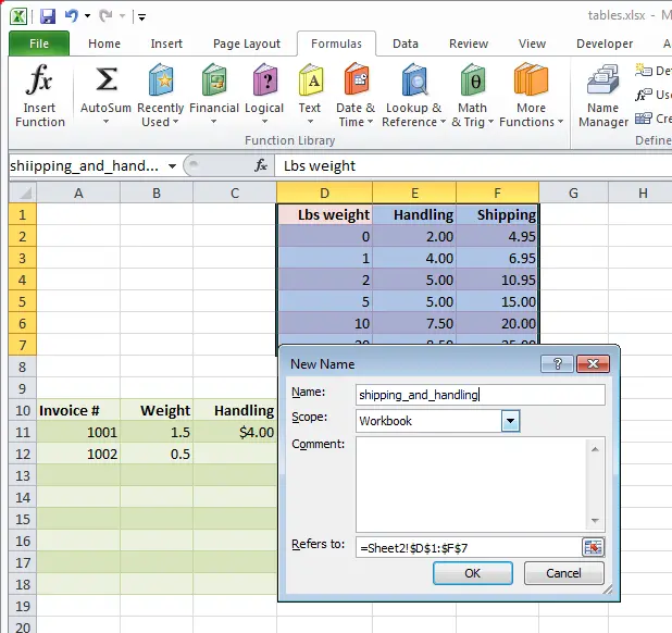
In addition, you can give your table a name, for this you need to select cells from D1 to F7 and press Formulas (formulas) > Define Name (Assign Name), then enter a name for the range and press OK. In our example, this is the name shipping_and_handling.
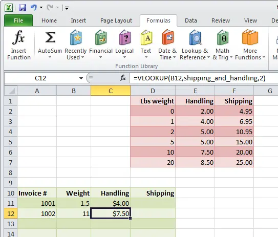
You can now use the range name when creating a formula. Here, instead of the address of the range, its name is indicated:
=VLOOKUP(B12,shipping_and_handling,2)
=ВПР(B12; shipping_and_handling;2)
We can adapt the formula from the column Action to calculate values in a column Shipping. In this case, only the column number will change. For Shipping Is the value 3:
=VLOOKUP(B12,shipping_and_handling,3)
=ВПР(B12;shipping_and_handling;3)
Function GPR works exactly the same way. More precisely, it also uses the search value and data range, but instead of the column number, you give it the row number. Lines are numbered 1, 2, 3 and so on, where 1 is the very first row of the table.
Using the previous example, we can match 11, 12, or 25 pounds, even though they are not in the table. The ability to find the nearest value that is less than the desired one looks very attractive. However, there are some caveats when using this formula. One of them is that the starting value in the table should be equal to 0which is actually what we have done. This allows errors to be avoided when a weight of, for example, less than 1 pound is used.
Working with Exact Matches
In some situations, you need to find an exact match with the value you are looking for, but there is no need for an approximate match. An example with carpet sizes and prices, which is shown in the figure below, just demonstrates this. If there is no carpet in the table Green weave, then there is no need to look for the next smaller value. In such a situation, we need either an exact match or an error message.
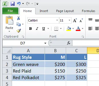
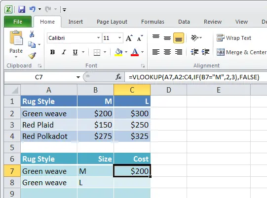
In this example, we look up the name in column A and return the price from column 2 or 3, depending on whether the specified carpet size is medium (M) or large (L). In this situation, we need to use the function IF (IF) to determine which column number to use. The search formula will look like this:
=VLOOKUP(A7,A2:C4,IF(B7="M",2,3),FALSE)
=ВПР(A7;A2:C4;ЕСЛИ(B7="M";2;3);ЛОЖЬ)
In this case, we are looking up the name of the carpet in column A and returning the price from column B or C, depending on the selected carpet size. If no exact match is found, i.e. the name of the carpet in the order does not match any of the names in column A, then an error message will be returned #AT (#N/A). Function IF (IF) is designed so that if the specified carpet size does not match one of the two available options, then the large size (L) will be taken by default.
Using data validation
In practice, it is desirable to make sure that the user enters the correct name of the carpet and its size. You can implement this using a drop down list. To do this, select the cells in which the user will enter their orders, for example, column A or B. Go to Data > Data Validation > Data Validation (Data > Data Validation > Data Validation). In the dialog box that appears, on the tab Settings (Settings) in the field Allow (Data type) select value List (List). Click in the field Source (Source) and select cells from A2 to A4, which contains a list with the names of carpets. Click OK.
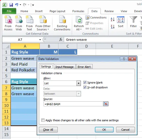
In the same way, you can create a drop-down list for entering dimensions. L or M, using a range as the data source B1: C1.
Now, when users select a carpet, they will be able to specify the desired options from the drop-down lists. This guarantees that the name will be specified without errors, since one of the positions present in the list will always be selected. In addition, if they change their mind and decide to choose a different carpet, then the function VPR will automatically recalculate and return the correct value.
Sorting data
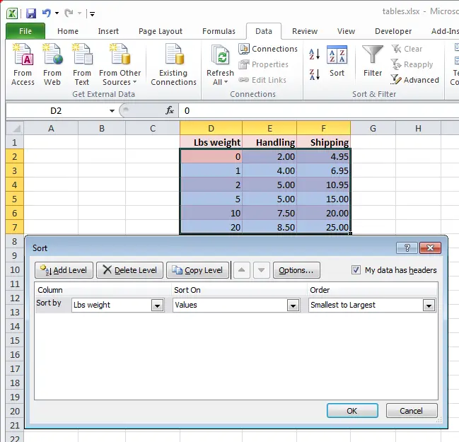
If you are working with approximate matches, you must sort in the table. To do this, select the entire data range, including the row headers in the first column. Column headings (header) can be omitted. On the tab Data (data) click command Black (Sort), a dialog box of the same name will open.
In line Sort By (Sort by) Specify sorting options. In the first drop-down list, select the column by which you want to sort, in our case it is the first column of the table. In the second select Values (Values), and in the third, specify the sort order in ascending order. If, along with the data, you have selected the table header, do not forget to check the box My data has headers (My data contains headers). Click OK.
The data table will be sorted so that the function VPR can work with it correctly.