


Contents
You might think that Excel is a spreadsheet program. This impression appears due to the fact that the worksheet is designed in the form of a grid, and the entered data really visually resembles a table. However, in Excel the concept of a table is somewhat different from the generally accepted one. What the average user calls a table is called a range in this program’s terminology.
Working with Excel tables differs from building tables in other electronic documents, such formats as Microsoft Word. And all this can scare a beginner a little. But, as they say, it was not the gods who burned the pots.
Benefits of Excel Spreadsheets
A normal sheet is just a set of cells that are identical in functionality. Yes, some of them may contain some information, others may not. But in general, they do not represent a single system from a program point of view.
A table, on the other hand, is not limited to a data range and is an independent object that has many characteristics, such as a name, its own structure, parameters, and a huge number of advantages over a regular range.
If you see the name “smart tables” in the course of further study of the topic, do not be embarrassed. This is the same as the table, these terms can be used as synonyms.
The main advantage of Excel tables is that when you add a new row to it, it automatically joins the table. This makes it possible to bind a table to a formula so that the formula automatically changes when new data is entered into the range.
The easiest way to understand the whole set of advantages of smart tables in practice. But first you need to learn how to create them.
Create an Excel table
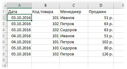
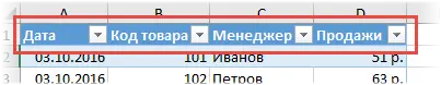
We have information about which manager was able to sell the product for what amount, written as a range from which to make a table.
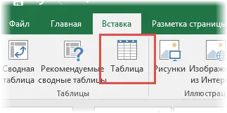
There are two ways to turn a range into a table. The first is to go to the “Insert” tab, and then click on the “Table” button.
The second is to use the hotkeys Ctrl + T. Next, a small window will appear in which you can more accurately specify the range included in the table, as well as let Excel know that the table contains headings. They will be the first line.
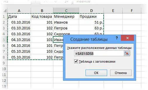
In most cases, no changes are required. After the OK key is pressed, the range will become a table.
Before you understand the features of working with tables, you need to understand how it works in Excel.
Basic features of working with tables
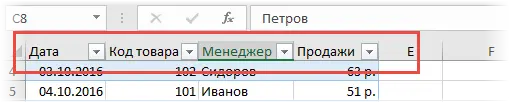
One of the most important elements of a table is its title. It can be seen in the Design tab. It is displayed immediately after the left mouse button is pressed on any cell included in it. The name is there, even if the user does not specify it. Just in this case, the default name is “Table 1”, “Table 2” and others.
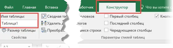
If you are going to use several tables at once in your document, then we recommend giving more descriptive names. In the future, it will then be much easier to understand which of them is responsible for what. This is especially important when working with Power Query and Power Pivot. Let’s name the table “Report”.
Excel has a separate function designed to see which tables and named ranges exist and quickly manage their names. In order to use it, you need to open the “Formulas” tab, and then find the “Name Manager” item.
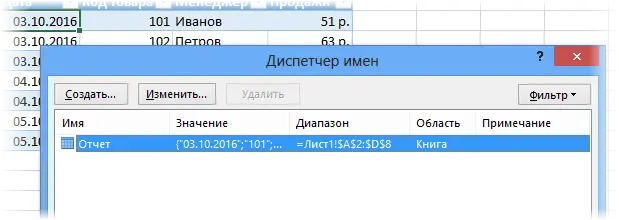
You can also see the name of the table when manually entering the formula.
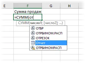
But most of all, it is curious that Excel can work not only with the table as a whole, but also with its individual parts – columns, headings, totals, and so on. To refer to a specific component, it is necessary to write formulas in this form.

A novice user will immediately say: “God, how can you learn all this”? But in fact, this does not need to be done, because hints appear during the typing of the formula. The main thing is not to forget to open the square bracket (it can be found in the English layout where we have the “x” button).
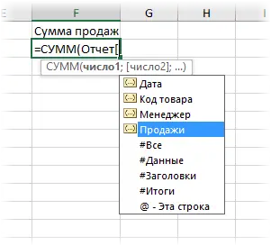
Switching between table components is done using the Tab key. After the formula is entered, do not forget to close all brackets, including the square one.
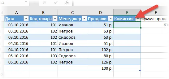
If in any cell you write a formula that returns the sum of the entire column “Sales”, then it will automatically take on this form.
=Report[Sales]
In simple words, the link does not point to a specific range, but to the entire column of the table.
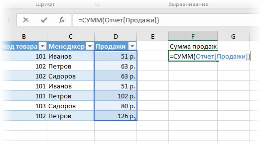
This suggests that if you use a smart table in a chart or pivot table, new information will be added there automatically.
Table properties
Excel spreadsheets can really make life easier. And one of the reasons for this is the ability to flexibly adjust its characteristics. Let’s look at how this can be done.
In addition to the main header, each table contains column headers, which are the values of their first row.
If the table is large, the user may still see the titles after scrolling down the range because the column titles in the coordinate bar are automatically renamed to the corresponding column titles.
If we were working with a regular range, we would have to separately fix the areas and sacrifice one line of the working field. Using tables saves us from this problem.
One of the functions of tables, which is added automatically when it is created, is the autofilter. It can be useful, but if it’s not needed, it’s easy to turn it off in the settings.
Here is a small demo of how a new row is automatically added to a table.
As we can see, new cells are automatically formatted to fit the table, and its cells are filled with the necessary formulas and links. Convenient, isn’t it?
The same goes for new columns.
If you insert a formula into at least one cell, it will automatically be copied to the entire column. Therefore, you do not need to manually use the autocomplete token.
But that’s not all. You can make certain changes to the functionality of the table.
Entering settings in the table
You can manage the table parameters in the “Designer” tab. For example, through the “Table Style Options” group, you can add or remove lines with headings and totals, make alternating line formatting, and bold the first or last paragraph.

Quickly make an attractive table design is not difficult thanks to ready-made templates. They can be found in the Table Styles group. If you need to make your own changes to the design, this is also easy to do.

The tools group allows you to perform some additional operations, such as creating a pivot table, removing duplicates, or deleting a table, turning it into a regular range.

But one of the most interesting features of any table is slices.
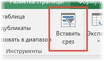
In simple words, this is a filter located on a separate panel. After clicking on the “Insert Slicer” button, we can select the columns that will serve as filtering criteria.

After that, a list of unique values of a certain column appears in a separate panel.
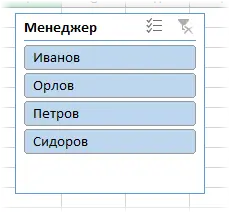
To apply a filter, you must click on the desired category.
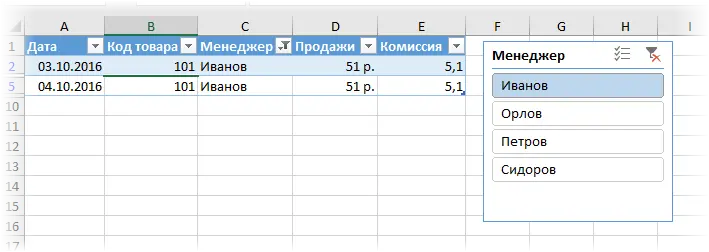
After that, only those values that correspond to the manager that was selected will be displayed.
You can also select multiple categories at once. This can be done by holding down the Ctrl key or by using the special button in the upper right corner, located to the left of removing the filter.
The cut can be customized. To do this, there is a separate tab on the ribbon called “Settings”. In it, the user can edit the appearance of the slice, the size of the buttons, the number of columns, and make a number of other changes. In general, everything is intuitively clear there, so any user can figure it out for himself.

But not everything is so simple…
The fact is that there are a number of shortcomings in Excel tables that impose certain restrictions on their work:
- There is no way to use views. In simple words, you cannot remember a number of sheet settings, such as a filter, collapsed rows or columns, and so on.
- You cannot use this book at the same time as another person through the sharing function.
- Only the insertion of the final totals is possible.
- Array formulas cannot be used in a table, which imposes serious restrictions when working with large amounts of data.
- Cells in a table cannot be merged. However, even in the normal range, this function is recommended to be used with caution.
- It is not possible to transpose a table so that the headings are in rows. To do this, it must be converted to a normal range format.
Some additional table features
Editing the values in the table is carried out in exactly the same way as in any other cell. If you enter duplicate values, Excel will prompt them in full after you enter one or more of the first characters.
The functionality of the tables provides for the possibility of automatic calculation of totals. To do this, select the desired column + one cell below it, in which the result will be displayed and click on the “Sum” button on the “Home” tab.
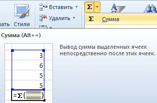
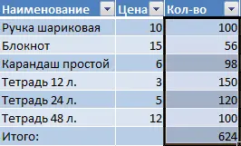
This is a standard Excel feature that is not directly related to tables. But since the value is displayed in the cell directly below this range, it is automatically added to the table. So it turns out that a separate column with totals is added.
One of the interesting features of smart tables is the use of numeric filters. They can be used to hide certain values. To access this function, as well as some other column parameters, just click on the arrow in the cell indicating the name of the column.

There you can also use options such as sorting by color, ascending or descending values, and a number of others.
Table and named range
One analog that will overcome some of the limitations described above is a named range. Of course, this is already a slightly different topic, since tables and named ranges intersect in a certain part of the functionality, but do not duplicate it.
It can also be referenced in a formula, as well as updating information in it. True, the latter will have to be done manually through the Name Manager.
Named ranges can be used in both simple and complex formulas. And in some aspects they can repeat the functionality of tables. For example, we have such a formula.
= СУММ(E2:E8)+СРЗНАЧ(E2:E8)/5+10/СУММ(E2:E8)
We see that here the same range (not a table and not named) is used several times at once. Suppose we need to change this range to some other one. In this case, changes will have to be made in three places at once.
If you assign a name to this range or turn it into a table, you just need to specify its name once, and then, in which case, just change the binding to a specific range also once.
Conclusions
Thus, smart spreadsheets in Excel open up a huge number of possibilities for the user. However, there are limitations, so the use of tables is not possible in all situations. If you want to leave a number of possibilities, but, for example, you need to transpose a range, then you need to convert the table into a named range, and then perform all the necessary actions.
Smart spreadsheets open up huge opportunities for the user to automate many Excel processes. But if you need to process a large amount of data, in some cases it is better to use a named range, to which you can apply array formulas and so on.