


Sharing Functions INDEX и MORE EXPOSED in Excel is a good alternative VPR, GPR и VIEW. This bundle is universal and has all the features of these functions. And in some cases, for example, when searching for data in a two-dimensional sheet, it will be simply irreplaceable. In this lesson, we will sequentially analyze the functions MORE EXPOSED и INDEX, and then look at an example of how to use them together in Excel.
Learn more about the VLOOKUP and VIEW functions.
SEARCH function in Excel
Function MORE EXPOSED returns the relative position of a cell in a given Excel range whose contents match the searched value. Those. this function does not return the content itself, but its location in the data array.
For example, in the figure below, the formula will return the number 5, since the name “Daria” is in the fifth line of the range A1:A9.
In the following example, the formula will return 3, since the number 300 is in the third column of the range B1:I1.
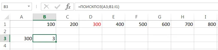
From the above examples, it can be seen that the first argument of the function MORE EXPOSED is the desired value. The second argument is the range that contains the value you are looking for. The function also has a third argument that specifies the type of mapping. It can take one of three options:
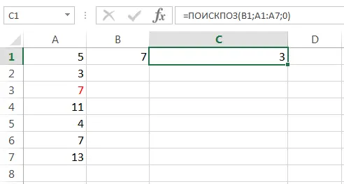
- 0 – function MORE EXPOSED searches for the first value exactly equal to the given one. Sorting is not required.

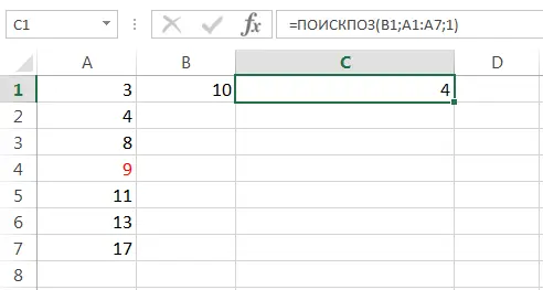
- 1 or completely omitted – function MORE EXPOSED searches for the largest value that is less than or equal to the given value. Sorting in ascending order is required.
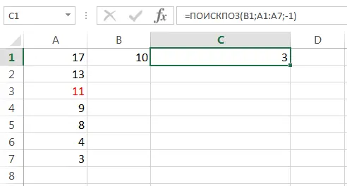
- -1 – function MORE EXPOSED searches for the smallest value that is greater than or equal to the given value. Sorting in descending order is required.
Alone function MORE EXPOSED, as a rule, is of little value, so in Excel it is very often used together with the function INDEX.
INDEX function in Excel
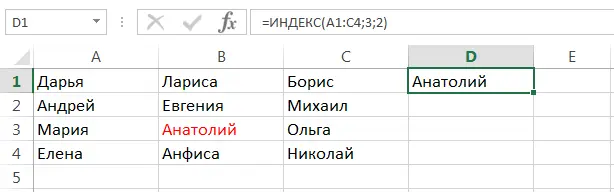
Function INDEX returns the contents of the cell that is at the intersection of the given row and column. For example, in the figure below, the formula returns a value from the range A1:C4, which is at the intersection of 3 rows and 2 columns.
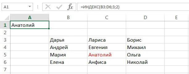
Note that the row and column numbers are relative to the top left cell of the range. For example, if the same table is placed in a different range, then the formula will return the same result:
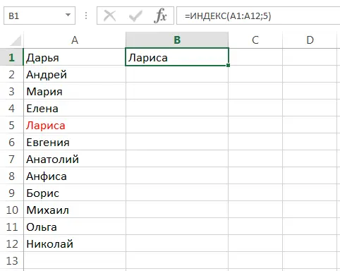
If the array contains only one row or one column, i.e. is a vector, then the second argument of the function INDEX specifies the number of the value in this vector. In this case, the third argument is optional.
For example, the following formula returns the fifth value from the range A1:A12 (a vertical vector):
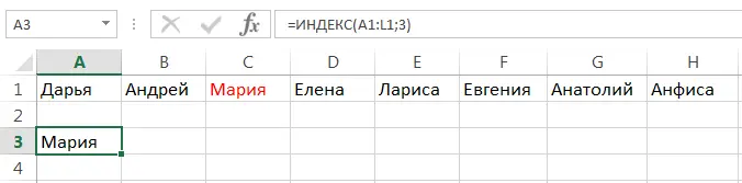
This formula returns the third value from the range A1:L1(horizontal vector):
Sharing MATCH and INDEX in Excel
If you have already worked with functions VPR, GPR и VIEW in Excel, they need to know that they are only searching in a one-dimensional array. But sometimes you have to deal with a two-dimensional search, when you need to search for matches by two parameters at once. It is in such cases that the connection MORE EXPOSED и INDEX in Excel is simply indispensable.
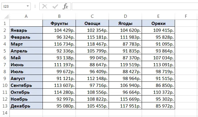
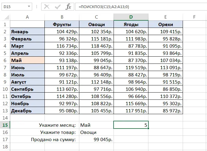
The figure below shows a table that contains the monthly sales of each of the four types of goods. Our task is to get the sales volume by specifying the required month and type of product.
Let cell C15 contain the month we specified, for example, May. And cell C16 is the type of product, for example, Vegetables. Enter the following formula in cell C17 and press Enter:
=ИНДЕКС(B2:E13; ПОИСКПОЗ(C15;A2:A13;0); ПОИСКПОЗ(C16;B1:E1;0))
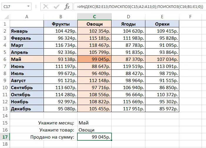
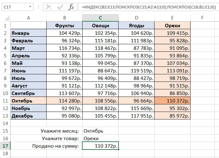
As you can see, we got the correct result. If you change the month and product type, the formula returns the correct result again:
In this formula, the function INDEX takes all 3 arguments:
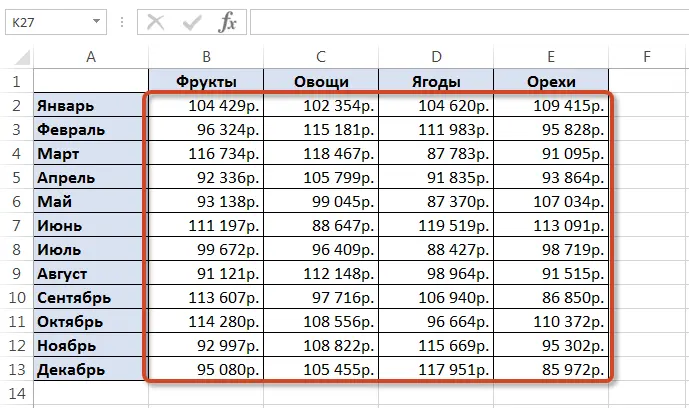
- The first argument is the range B2:E13 in which we are searching.
- The second argument of the function INDEX is the line number. We get the number using the function MATCH(C15;A2:A13;0). For clarity, we calculate what this formula returns to us:
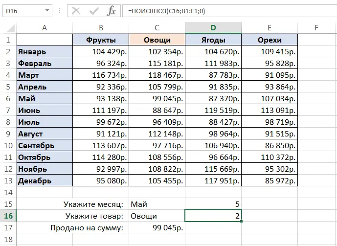
- The third function argument INDEX is the column number. We get this number using the function SEARCH(C16;B1:E1;0). For clarity, we calculate this value:
If we substitute into the original cumbersome formula instead of functions MORE EXPOSED already calculated data from cells D15 and D16, then the formula will be transformed into a more compact and understandable form:
=INDEX(B2:E13;D15;D16)
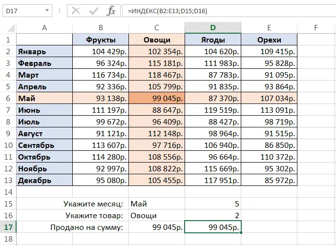
As you can see, everything is quite simple!
On that beautiful note, we will end. In this lesson, you got acquainted with two more useful features of Microsoft Excel – MORE EXPOSED и INDEX, analyzed the possibilities on simple examples, and also looked at their joint use. I hope this lesson was helpful to you. Stay tuned and good luck learning Excel.