Contents
Problem
If you are building several pivot tables based on the same source, then you may have already encountered one small but unpleasant moment: Excel does not allow you to independently group data in such pivot tables.
Let’s say we built two separate pivot tables to analyze revenue and sales volumes:
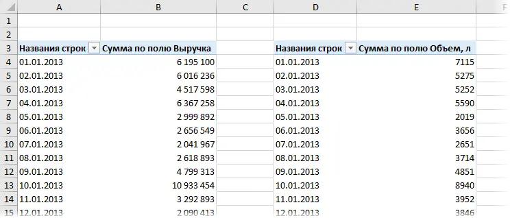
But we want to see the revenue by months, and the sales volume by quarters, so it is logical to apply the grouping further. Right-click on the dates in the first summary, select Group – Months – OK and the revenue really starts to be displayed by months, as we wanted. But in the second table, the dates were also grouped by months, although we did not ask for this at all:
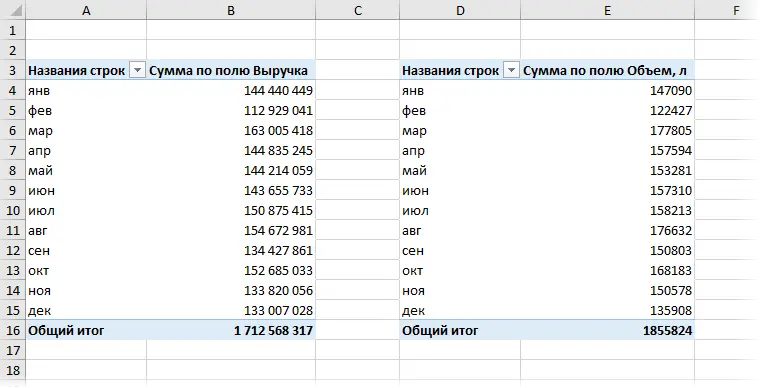
And vice versa, if you try to group the dates in the second summary by quarters in a similar way, then the first summary will also be regrouped, losing the current grouping by months.
What is it?
The fact is that when building any pivot table, Microsoft Excel creates a so-called cache (Pivot Cache) in the file – a memory area where the initial data is loaded for analysis and calculations. And when you do the second, third, etc. pivots for the same source table Excel helpfully uses the previously generated cache for the first pivot, rather than creating a new one.
On the one hand, this is correct: the data is not duplicated, the file weighs less and is calculated faster. On the other hand, we have the same grouping problem, a change in which in one of the pivots affects all the others. What to do?
Method 1. We build the summary correctly
To build a pivot table on the new cache, you will have to use the good old PivotTable and PivotChart Wizard (Pivot Table and Chart Wizard) from versions of Excel 97-2003. Oddly enough, but this “outdated” tool can choose when creating a summary – whether to make an independent summary or a summary based on an existing cache. The button for this Wizard was removed from the interface back in 2007, but it is still available for compatibility and is quite functional.
Right-click on the quick access toolbar in the upper left corner and select command Customizing the Quick Access Toolbar (Customize Quick Access Toolbar). Then, from the drop-down list at the top of the window, select All teams (All Commands), find PivotTable and PivotChart Wizard and add to the panel:
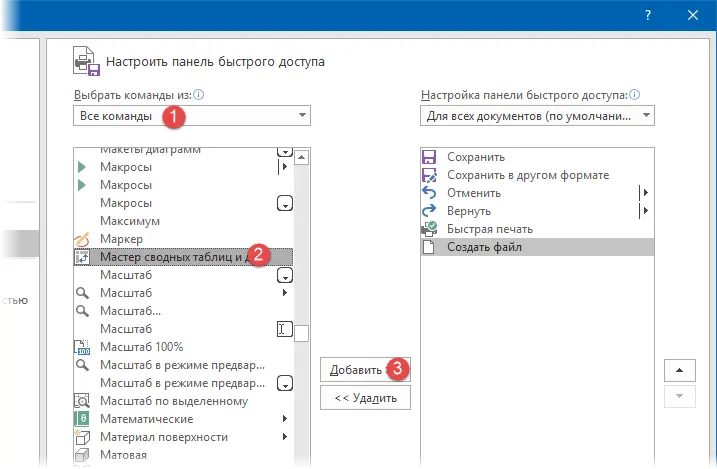
Now you can build a summary. We put the active cell in the table with data or select it, click on the added button and go through the steps of the Wizard, choosing first to create an independent report on our own cache:

Excel will persistently offer to make a summary on the same cache – we refuse and reach the final:

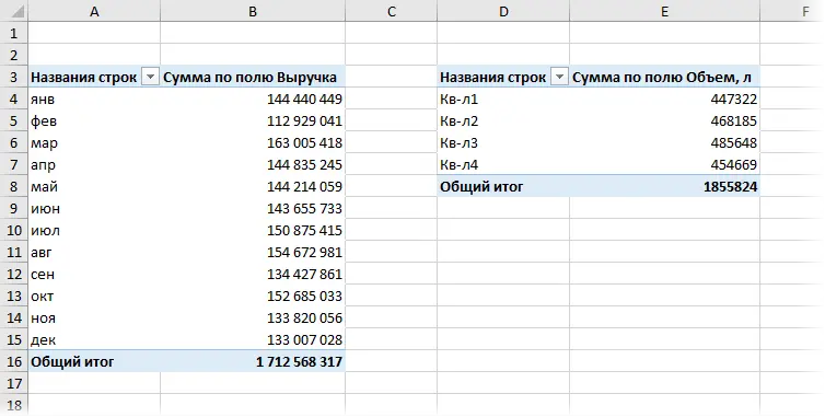
That’s it, now the grouping of this pivot will not affect the neighboring one, and both tables can be grouped differently:
Method 2. We untie the already created summary from the general cache
If you already have a ready-made summary, and you don’t want to create it again using the Wizard, then you can unlink it from the general cache using a tactical trick:
- Copy the summary to a new empty file
- Update the summary (right-click on it – Update & Save)
- Copy it back to the old location
Such a meaningless, at first glance, “feint with the ears” makes Excel create a separate copy of the cache for the summary, i.e. makes her independent.
If such an operation will have to be done often, then it makes sense to automate this with a small macro. Click the button Visual Basic tab developer (Developer) or keyboard shortcut Alt + F11to open the Visual Basic Editor, then insert a new empty module via the menu Insert – Module and copy this code there:
Sub Unlink_Pivot_From_Shared_Cache() Dim pvtTable As PivotTable Dim startcell As Range Dim wbCur As Workbook, wbTemp As Workbook On Error Resume Next Set pvtTable = ActiveSheet.PivotTables(ActiveCell.PivotTable.Name) On Error GoTo 0 If Not pvtTable Is Nothing Then Set wbCur = ActiveWorkbook 'copy the pivot and paste it into a new workbook Set startcell = pvtTable.TableRange2.Cells(1) pvtTable.TableRange2.Copy Set wbTemp = Workbooks.Add ActiveSheet.Paste 'update the pivot, copy back and close the temporary file ActiveSheet.PivotTables(1) .PivotCache.Refresh ActiveSheet.PivotTables(1).TableRange2.Copy Destination:=startcell wbTemp.Close SaveChanges:=False Else MsgBox "Put active cell in pivot table first!", vbExclamation, "Hint" End If End Sub
If you put the active cell in the summary and run this macro using the button Macros tab developer or keyboard shortcuts Alt + F8, then the current pivot table will be decoupled from the shared cache, and you can group it independently.
Nuances
- If pivot tables do not have a shared cache, then they cannot be filtered by slicers and scale at the same time.
- You can see the number of caches in a book if you use the Visual Basic editor (Alt + F11) open console via menu View — Immediate and enter the command there ? Activeworkbook.PivotCaches.Count and click on Enter:

- Fine-Tuning PivotTable Calculations
- Source data filter when double clicking on a cell in a pivot table
- Grouping data in pivot tables


