How to work with pivot tables in Excel (with examples)

If you need to turn a huge amount of data into a concise report within a short time, you can use an Excel tool such as pivot tables. In addition, they make it possible to carry out analysis by different methods by simply dragging fields from one area to another. Unfortunately, a large number of users cannot fully appreciate this tool. As a rule, they do not understand the full range of opportunities that it provides them.

How pivot tables are useful

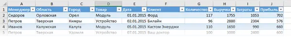
Let’s imagine that there are no pivot tables at all. Suppose you are employed in an organization that sells certain products. Their assortment is small – only 4 pieces. And only a few dozen buyers from different areas carry out orders. After the sale of the goods has been carried out, the data is entered in a separate line.

From time to time, the boss sets the task of creating a summary report based on this data, distributed across different regions. To complete it, you must first make a table header, in which only the values ​​uXNUMXbuXNUMXbof products and regions will be entered. After that, a copy of the column with products is created, and duplicates are removed.

Next, you need to transpose the column into a row. The same actions are performed on areas, only transposition is not used. As a result, you will get such a header for the future report.

This table must be filled in, that is, you need to find out the amount of revenue from the desired regions for each of the commodity items. This task is easily accomplished using the function SUMMESLIMN. In addition, you need to add totals. After that, a summary report for each area will appear. 

Hooray, now you are satisfied and are reporting to the boss, who took a look at him and asked him to implement a number of more ideas:

1. When compiling a report, use not revenue, but profit. 

1. Show by columns – regions, and by rows – products.
2. Make similar reports for each manager separately. 

To complete this task, you will have to spend a lot of time even if your level of professionalism is quite high. At the same time, there is a high risk of making many mistakes. You can prevent them with a pivot table. Then these tasks can be completed in just five minutes (and with proper experience, even faster).

Create an Excel PivotTable

Let’s start by opening the file or sheet where the source information is located. A pivot table may well be created based on a standard range, but it is much better to first convert to a table format. In this way, you can immediately remove the need to update the original range each time you add new data.

Next, we should select any cell you want and open the “Insert” tab. On the left side of the ribbon there are two items “Pivot Table” and “Recommended Pivot Tables”.

The second option is needed for those people who do not know how the final result should look like. Based on what data is entered in the range, Excel will offer several options. The user can only choose the one that suits him best.

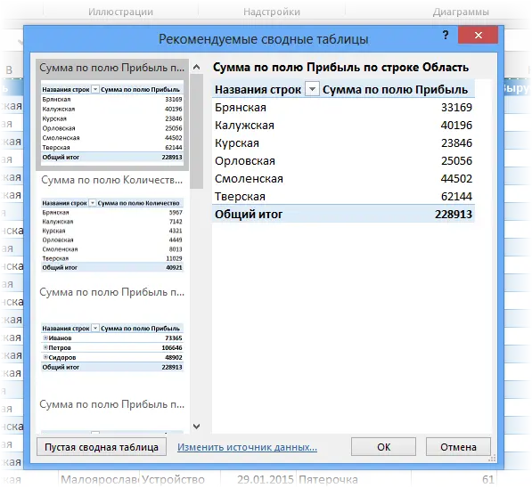
After clicking on the required option, the table will be automatically generated. It remains only to make a few elementary changes so that the final result matches the preferences of a particular person as much as possible.

It may also be a task to make a pivot table yourself. In this case, you must click on the usual button “Pivot Table”. In the window that appears, you must enter the range that will be used to create the pivot table and its location (the standard option is a new sheet).

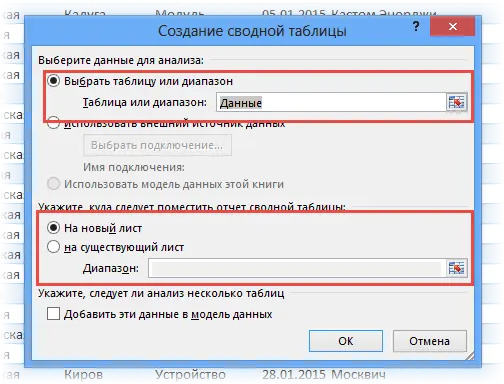
As a rule, no additional changes are required at this stage. After the user confirms the actions by pressing the “OK” key, a pivot table layout will appear on a new sheet, which does not yet contain any data.

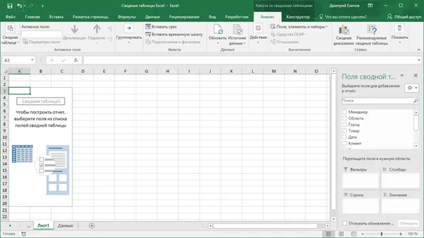
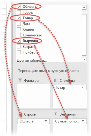
To customize it, you need to use the PivotTable Fields panel located on the right side of the sheet.

Above it is a list of all fields that can be used. They are columns in the original range. If you need to add another field to the layout, just put a tick in the appropriate place. The location of the Excel field, as a rule, determines itself. But in some cases it fails. Then the problem is solved by simply dragging the mouse to the desired location.

To remove a field, simply clear the corresponding checkbox.

Composite Components

The PivotTable contains the following components:

1. Value area. It means the main part of the table with values. Excel gets them by aggregating the source data using the method that the user chooses. Typically, this is done using Summation. This method is set automatically, provided that all data in the source range is in a cell that has a number format. If at least one cell contains text or there is no information, then the number of cells will be automatically calculated. There are about 20 different types of calculations in total. the easiest way to change it is by right-clicking on any cell of the required field of the pivot table and choosing the aggregation method.
2. Row area. Actually, this includes the names of the lines located in the leftmost column. These are all column values ​​that are unique in their kind and have been selected by the user. There may be several fields here. Such a table is called multilevel. As a rule, any non-quantitative data is located here, such as the names of products, regions, and so on.
3. Column area. The same as the rows area, only for the columns. This can include years, months, and product groups.
4. Filter area. It is used to show only certain values ​​that correspond to a specific attribute. For example, it is possible to display data only for a specific industry, for a certain period, and so on. In this case, you need to place the filter field in the filter area and select the required value from the drop-down list. 

It is the filter area that allows you to make flexible settings for the data slice. In theory, it all sounds a little confusing. Let’s do everything on a specific example. Let’s make the same table as above. To do this, drag the “Revenue” field to the “Values” area, “Region” to the “Rows” area, and “Product” to the “Columns” area.

After that, we will see a full-fledged pivot table.

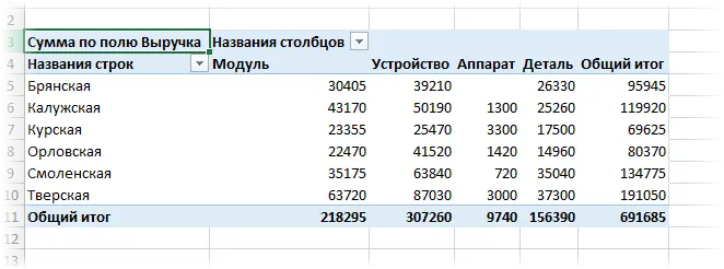
And what is surprising? It took only 10 seconds to create it. 

PivotTable Operations

Editing a PivotTable is as simple a task as creating one. Let’s see how the ideas that the director proposed above are implemented in practice.

Let’s replace revenue with profit.

With a simple drag and drop, you can swap products and areas.

In our case, we used the filter area, where we placed the “Manager” field.

There are several other methods for filtering data, but this one is the main and the simplest. That’s it, just a few seconds are enough to complete this simple task.

This is how the user interacts with pivot tables in Excel. Of course, in practice, things can be much more complicated than in these simple examples. For example, sometimes you have to use a more tricky way of aggregation, add fields, conditional formatting, and so on. But if you have at least a little knowledge, all this will not be difficult to implement.

Useful tips for choosing a data source

To perform PivotTable tasks most effectively, the source data must meet a number of criteria. It is very important that there is a title above each column to identify what the data is. In addition, follow these helpful tips:

1. It is best to use a smart table as a data source. Its main advantage is that each column has its own name, and if you add columns or rows, the data range is automatically expanded by their corresponding number.
2. It is not recommended to repeat groups in columns. So, it is desirable that the dates are located in one column, and not broken down by months in separate columns.
3. Format the fields correctly. It is important that all numbers are in numeric format and dates are valid in date format. Otherwise, it will be difficult for Excel to correctly group and process the data. In principle, Excel automatically determines the data type, but in some cases glitches are possible. Therefore, before creating a pivot table, you need to make sure that all the information in the source is in the correct format. 

How to update data in a pivot table

The PivotTable is not automatically updated. Therefore, in order to update it, after each change in the source, it is necessary to right-click on it and press the “Update” button in the menu that appears.

You can also perform a similar operation through the Data tab on the ribbon. To do this, just click on the “Update All” button, highlighted with a red rectangle in the screenshot.

This seems to be inconvenient, and it would be much better to do an automatic update. But in fact, in this case, too much RAM would be wasted. To save computer resources, work is carried out not directly, but through an intermediary link in the form of a cache. 

How to create a dashboard in Excel

Once a person masters the technique of creating pivot tables, he can proceed to another way of displaying summary data, which is built on them. Dashboards are a very handy way to visually present information based on a specific range of data.

Of course, creating dashboards is not as simple a task as generating smart tables, but it allows you to make the right impression both on your bosses, and on investors or any other interested parties.

As a rule, in companies, the creation of smart tables is limited, while dashboards have a huge number of advantages:

1. It gives you the opportunity to flexibly manage report elements, focusing on the most relevant indicators or replacing them if necessary.
2. It makes it possible to compactly fit all the necessary information literally on one sheet, which allows you to save paper if the authorities require you to print reports. 
3. With the help of dashboards, it is easy to compare key indicators for different periods. 

Among other things, the ability to work with dashboards speaks of the professionalism of the employee. Such a skill immediately raises him head and shoulders above in the eyes of management.

There are many ways to create Excel dashboards, but you should always start with sketches right on a piece of paper. It is necessary to draw which blocks will be located in which places. Next, it will be much easier to create a dashboard. In particular, you can create a dashboard in Excel using the PowerView add-in. Also, visualization can be carried out by such methods:

1. Shapes and Word Art objects. They allow you to draw anything, up to engineering drawings. In addition, there are many text labels that allow you to describe any component of the dashboard.
2. Using pivot tables.
3. Graphs that can also use the original range as data.

All of them can be used to create dashboards. Moreover, thanks to these visualization tools, you can do them literally in a short time.

Conclusions

Thus, creating pivot tables in Excel is not a difficult task at all, which will save many hours when creating reports. It is enough to press just a few buttons, and the reporting table will be created automatically. Then it can be edited and customized. Good luck.