


Contents
Some time ago, we published the first part of our tutorial on creating charts in Excel for beginners, which gave detailed instructions on how to create a graph in Excel. And the very first question asked in the comments was:How to show data on different worksheets in a chart?“. I want to thank the reader who asked this wonderful question!
In fact, the source data that needs to be shown on the diagram is not always located on the same worksheet. Fortunately, Microsoft Excel allows you to display data located on two or more sheets on one graph. Next, we will do this step by step.
How to Create a Chart from Multiple Excel Sheets
Let’s assume that several Excel sheets contain income data for several years, and you want to plot a chart on this data to show the overall trend.
1. Create a chart from the data of the first sheet
Open the first Excel worksheet, select the data you want to display in the chart, open the tab Insert (Insert) and in section Diagrams (Charts) select the desired chart type. For our example, we will choose Volumetric Stacked Histogram (Stack Column).
2. Add a second row of data from another sheet
Click on the chart you just created to bring up a group of tabs on the Menu Ribbon Working with charts (Chart Tools), open the tab Constructor (Design) and press the button Select data (Select Data). Or click on the icon Chart Filters (Chart Filters) to the right of the chart and at the very bottom of the menu that appears, click the link Select data (Select Data).
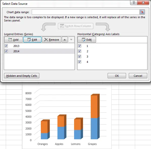
In the dialog box Selecting a data source (Select Data Source) button Add (Add).
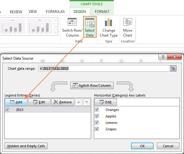
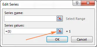
Now let’s add a second row of data from another worksheet. This point is very important, so follow the instructions carefully. After pressing the button Add (Add) dialog box will open Row change (Edit Series), here you need to click the range selection icon next to the field The values (Series values).
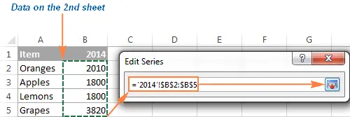
Dialog window Row change (Edit Series) will collapse. Click on the sheet tab containing the next piece of data to be shown in the Excel chart. When switching to another sheet, the dialog box Row change (Edit Series) will remain on the screen.
On the second sheet, select the column or row of data you want to add to the Excel chart, and click the range selection icon again to bring up the dialog box. Row change (Edit Series) returned to the original size.
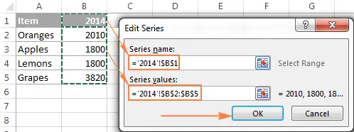
Now click on the range selection icon next to the field Row name (Series name) and select the cell containing the text you want to use as the name of the data series. Click the range selection icon again to return to the original dialog box. Row change (Edit Series).
Check the links that have now appeared in the fields Row name (Series name) и The values (Series values), and press OK.
As you can see in the picture above, we have linked the row name to the cell B1A that contains the column heading. Instead of referring to a column heading, you can enter the name as a text string enclosed in quotation marks, for example:
="Второй ряд данных"
The data series names will appear in the chart legend, so it’s best to come up with meaningful and descriptive names. At this stage, the result should look something like this:
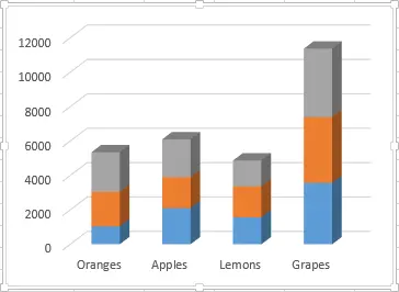
3. Add more data series (optional)
If the chart needs to show data from more than two worksheets, then repeat the previous step for each data series that you want to add to the chart. When you’re done, click OK in the dialog box Selecting a data source (Select Data Source).
I added a third data series as an example, and my chart now looks like this:
4. Customize and enhance the chart (optional)
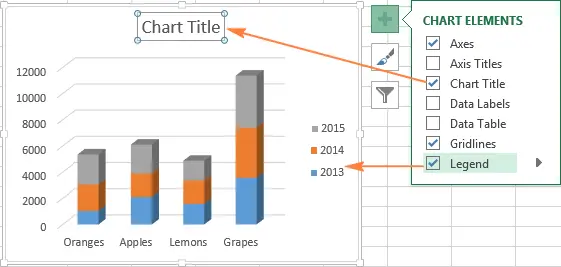
When you create charts in Excel 2013 and 2016, elements such as the chart title and legend are usually added automatically. Our multi-sheet chart didn’t have a title and legend added automatically, but we’ll fix that quickly.
Highlight the chart, click the icon Chart elements (Chart Elements) in the form of a green cross near the upper right corner of the chart, and check the boxes for the options you need:
How to customize other chart options, such as the display of data labels or the format of the axes, is described in detail in a separate article on customizing Excel charts.
Create a chart from a summary table
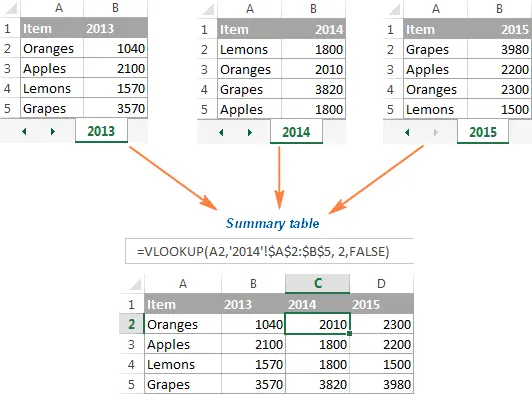
The solution shown above is only useful if the data to be displayed on the chart is in the same order on all worksheets, i.e. in the first line – Oranges, in the second – Apples etc. Otherwise, the graphs will turn into something illegible.
In this example, the layout of the data is the same on all three sheets. If you need to build a graph from much larger tables, and there is no certainty that the data structure in these tables is the same, then it would be wiser to first create a final table, and then create a chart from the resulting final table. To fill the final table with the desired data, you can use the function VPR (VLOOKUP).
For example, if the worksheets in question in this example contain data in a different order, then we can make a summary table out of them using the following formula:
=ВПР(A3;'2014'!$A$2:$B$5;2;ЛОЖЬ)
=VLOOKUP(A3,'2014'!$A$2:$B$5,2,FALSE)
And get this result:
Next, just select the final table, open the tab Insert (Insert) and in section Diagrams (Charts) select the desired chart type.
Setting up a chart in Excel created from several worksheets
It may happen that after completing the creation of a diagram from two or more worksheets, it becomes clear that it should be built differently. And since creating such a chart in Excel is not as fast a process as creating a chart from a single sheet, it is likely that it will be easier to redo the created chart than to create a new one from scratch.
In general, the options for an Excel chart created from multiple worksheets are the same as the options for a regular Excel chart. You can use a group of tabs Working with charts (Charts Tools), or the context menu, or the settings icons in the upper right corner of the chart to customize basic elements such as chart title, axis titles, legend, chart style, and more. For step-by-step instructions on how to customize these options, see Customize charts in Excel.
If you want to change the data series shown in the diagram, then you can do this in one of three ways:
Modifying a Data Series Using the Select Data Source Dialog Box
Open a dialog box Selecting a data source (Select Data Source), for this on the tab Constructor (Design) click Select data (Select data).
To change a data series, click on it, then click the button Change (Edit) and edit the parameters Row name (Series Name) or Value (Series Values) as we did earlier in this article. To change the order of data series in a chart, select the data series and move it up or down using the corresponding arrows.
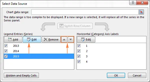
To hide a row of data, simply uncheck the list Legend elements (Legend Entries) on the left side of the dialog box. To remove a data series from the chart completely, select it and click the button Remove (Remove).
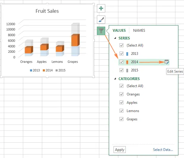
Hide or show data series using the Chart Filters icon
Another way to manage the data series that are displayed in an Excel chart is with the icon Chart Filters (Chart Filters). If you click on the diagram, then this icon will immediately appear on the right.
- To hide data, click on the icon Chart Filters (Chart Filters) and uncheck the corresponding data series or category.
- To change the data series, click the button Change row (Edit Series) to the right of the series name. The familiar dialog box will appear. Selecting a data source (Select Data Source), in which you can make the necessary settings. To button Change row (Edit Series) has appeared, just hover over the name of the series. In this case, the data series that the mouse is hovering over is highlighted in the diagram in order to make it easier to understand which element will be changed.
Changing a data series using a formula
As you probably know, every row of data in Excel is defined by a formula. For example, if you select one of the data series in the chart we just created, the data series formula will look like this:
=РЯД('2013'!$B$1;'2013'!$A$2:$A$5;'2013'!$B$2:$B$5;1)
=SERIES('2013'!$B$1,'2013'!$A$2:$A$5,'2013'!$B$2:$B$5,1)
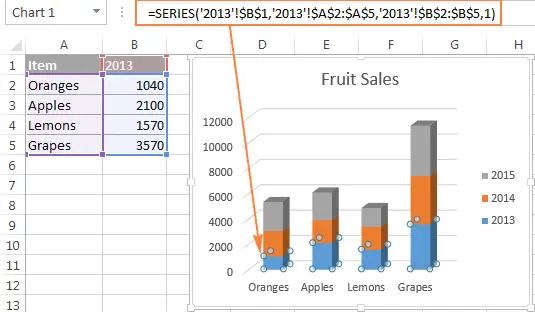
Each data series formula consists of several basic elements:
=РЯД([имя_ряда];[имя_категории];диапазон_данных;номер_ряда)
That is, our formula can be decoded as follows:
- Series name (‘2013’!$B$1) taken from cell B1 on the sheet 2013.
- Category names (‘2013’!$A$2:$A$5) taken from cells A2: A5 on the sheet 2013.
- Data (‘2013’!$B$2:$B$5) is taken from cells B2: B5 on the sheet 2013.
- The row number (1) indicates that this row occupies the first place on the chart.
To change a specific data series, select it in the chart and make the necessary changes in the formula bar. Of course, you need to be very careful when changing the formula of a data series, since it is easy to make a mistake, especially if, during editing, the source data is contained on different sheets, and not in front of your eyes. However, if working with formulas is more convenient for you than with the usual interface, then this way to make small corrections may well be suitable.
That’s all for today! Thank you for your attention!