How to quickly calculate totals in an Excel spreadsheet

When maintaining most tables in Excel, after some time, you need to calculate the total of individual columns or the entire working document. However, if you do it manually, the process can take several hours, and it’s easy to make mistakes. To get the most accurate result and save time, you can automate your actions through the built-in tools of the program.

Ways to calculate totals in a worksheet

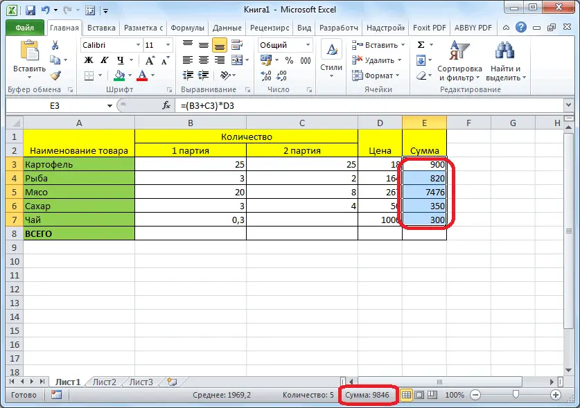
There are several proven ways to calculate totals for individual columns of a table or multiple columns at the same time. The easiest method is to select values ​​with the mouse. It is enough to select the numerical values ​​​​of one column with the mouse. After that, at the bottom of the program, under the sheet selection line, you can see the sum of the numbers from the selected cells.

If you need to not only see the final sum of numbers, but also add the result to the worksheet, you must use the autosum function:

1. Select the range of cells whose sum total is to be obtained.
2. On the “Home” tab on the right side, find the autosum icon, click on it.

3. After performing this operation, the result will appear in the cell under the selected range.

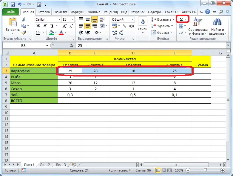
Another useful feature of AutoSum is the ability to get results under multiple adjacent columns of data. Two scoring options:

1. Select all cells under the columns, the sum of which you want to get. Click on the autosum icon. The results should appear in the highlighted cells.
2. Mark all columns from which you want to calculate the total, along with empty cells below them. Click on the autosum icon. The result will appear in free cells.

Important! The only disadvantage of the AutoSum function is that it cannot be used to calculate the totals of individual cells or columns that are located far from each other.

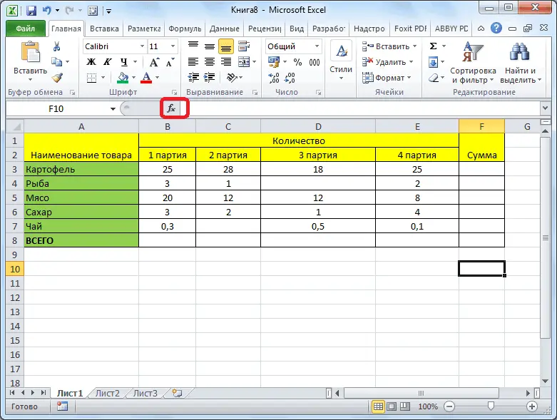
To calculate results for individual cells or columns, you must use the “SUM” function. Procedure:

1. Mark by pressing LMB the cell where you want to display the result of the calculation.
2. Click on the add function symbol.

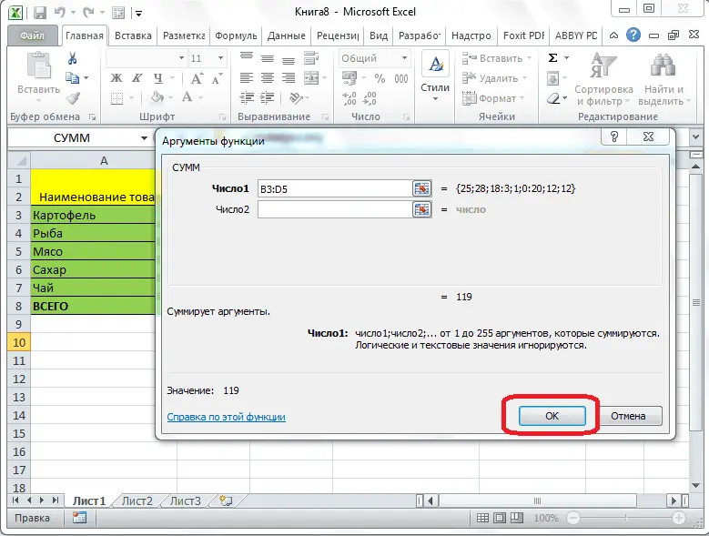
3. This should open the “Function Wizard” setup window. From the list that opens, select the required function “SUM”.
4. To exit the “Function Wizard” window, click the “OK” button.

Next, you need to set up the function arguments. To do this, in the free field you need to enter the coordinates of the cells, the sum of which you want to calculate. In order not to enter data manually, you can use the button to the right of the free field. Below the first free field is another empty line. It is designed to perform the calculation for the second data array. If you need information for only one range of cells, you can leave it empty. To complete the procedure, click on the “OK” button.

How to calculate subtotals

One of the common situations that people who actively work in Excel spreadsheets face is the need to calculate subtotals in one worksheet. As with the grand total, this can be done manually. However, the program allows you to automate your actions, quickly get the desired result. There are several requirements that a table must meet in order to calculate subtotals:

1. When creating a column heading, you cannot enter multiple lines in it. At the same time, the header should be located on the first line of the worksheet.
2. It is not possible to get subtotals in columns containing empty cells. Even if there is one empty cell in the entire table, the calculation will not be performed.
3. The working document should have a standard range without formatting.

The process of calculating subtotals itself consists of several steps:

1. First of all, you need to distribute the data in the first column so that they are distributed into groups of the same type.
2. Left-click to select any arbitrary cell of the worksheet.
3. Go to the “Data” tab on the main page with tools.
4. In the “Structure” section, click on the “Subtotals” function.
5. After performing these actions, a window will appear on the screen in which it is necessary to prescribe the parameters for further calculation.

In the “Operation” parameter, you must select the “Sum” section (it is possible to select other mathematical operations). In the next parameter, specify the columns for which subtotals will be calculated. To save the specified parameters, click the “OK” button. After performing the steps described above, between each group of cells, one intermediate will appear, in which the result obtained after the calculation will be indicated.

Important! Another way to get subtotals is through a separate function “SUBTOTALS”. This function combines several calculation algorithms that must be entered in the selected cell through the function line.

How to remove subtotals

The need for the existence of intermediate results completely disappears over time. So that extra values ​​do not distract a person during work, the table received its original integrity, you need to delete the calculation results with their additional lines. To do this, you need to perform several actions:

1. Go to the “Data” tab on the main page with tools. Click on the “Subtotal” function.
2. In the window that appears, check the “Size” item, click on the “Remove All” button.
3. After that, all added data, along with additional cells, will be deleted.

Conclusion

The choice of how to obtain the results of the Excel worksheet directly depends on where the data required for the calculation is located, whether the results need to be entered in the table. After answering these questions, you can choose the most appropriate method from those described above, repeat the procedure according to the detailed instructions.