How to put a discount on a product in an Excel spreadsheet (discount formula)

Excel is used for various purposes, including monitoring discounts for certain customers. Let’s imagine a situation, we have a range of data describing different buyers. Our task is to offer each of them a discount, but its size will depend on the available material possibilities of buyers.

This task can be implemented using a data table. Let’s take a closer look at how it is created, how it can be used, and give specific cases of how it all works. 

Using a Data Table in Excel

In order to understand the issue in more detail, you must first understand what a data table is. This is a kind of simulator that represents different situations, observes the change in values ​​and, based on the resulting data, shows what effect they will have on the final result.

That is, it is, to a certain extent, artificial intelligence that can be used for our purposes. Our version of the simulator will look at what values ​​are placed in the cells, and based on this information, indicate what the final result will be in the end.

This is a way to quickly understand what the possible outcomes are. It is enough to set only two variables, after which the program will automatically select a huge number of results, and we just have to choose the most optimal of them.

There are a huge number of advantages that this tool has. One of them is that all results are located within one sheet. This is very convenient if you need to quickly understand the current situation and draw conclusions based on the current picture.

How to create a data table in Excel

To create a data table in Excel, you first need to build two models:

1. The company’s profit model and the terms of the affiliate program.
2. A data scheme that will somewhat resemble a Pythagorean table. We want the row to display quantitative values ​​for each bonus that is offered under this program. For example, they can be a set of numbers from 100 to 500, which are divisible by 50. And the bonus itself as a percentage should be measured, for example, within 3-10 percent, and most importantly, that they be a multiple of 5.

It is important to note that in the case of an intersection of a column and a row, the cell located at this intersection should not contain any data. 

Now in the cell located at the intersection, enter the formula, = B15 / B8. Don’t forget that the cell format must be percentage. 

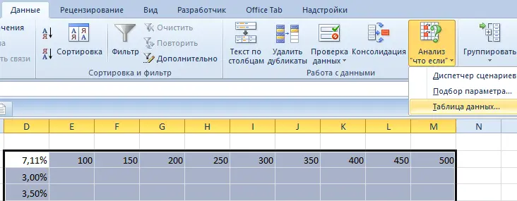
The next step is to select the range D2:M17. Next, we need to select the “Data” tab to create a table (this is where all the necessary settings are located). On this tab, we need to use the “Analysis: What If” tool and find the “Data Table” item there. The tool itself is located in the “Work with data” group.

After pressing this menu, a window appears where you need to write the correct data ranges. They can also be selected manually by clicking on the special button to the right of the input field. 

In our case, the rules are:

1. The upper field contains an absolute link to the cell that indicates the boundary level of bonuses.
2. In the bottom field, write down the range with percentage bonuses.

You can see the ranges that we use in this example in this screenshot.

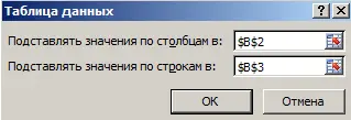
It is important to take into account that we calculated the most optimal offers with indicators of the second limit for quantitative limit 1. If we need to calculate discounts for the second quantitative limit, then we need to indicate links to other cells. In our case, these are $B$4 and $B$5.

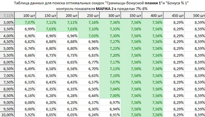
After we confirm our actions, the table will be automatically filled with the necessary data. In our case, it turned out to automatically display 135 possible options. And nothing needed to be sorted out manually. Convenient, isn’t it?

Don’t forget to set the percentage cell format for the options.

Datasheet analysis with visualization (what if)

Here we have a question: do we need to analyze the data manually later? After all, a computer is unlikely to be able to understand our tasks so well. To a certain extent, yes. But you can simplify this process somewhat with the help of visualization. 

How to do it? For this purpose, there is a tool called Conditional Formatting. The sequence of actions is as follows:

1. We find the required range with the cursor and select it. In our case, this is a set of cells E3:M17.
2. Next, we need to select the “Between” rule in the “Conditional Formatting” section.
   

   

3. We set the percentages that interest us. In our case, these are values ​​ranging from 7 to 8 percent. In the right part of the window, you can select the formatting style that will be used to highlight matches.

Now the income corridor is shown automatically. We know that exiting it is fraught with loss of profit. The user can then easily understand what size of the discount is optimal in a particular situation, so that it is beneficial for both the buyer and the seller. And with the help of conditional formatting, this is generally easy. 

That is, we have calculated the most correct discount in a particular situation.

A similar method is used to calculate bonuses and levels for the second border. Just do not forget to indicate the correct links for each specific case. 

The table for net profit is constructed in exactly the same way. We can set the appropriate conditional formatting in this case.

In this way, you can immediately take into account the optimal discounts in the budget and get the maximum profit due to the greatest loyalty of the target audience. 

When we communicate with clients, bonuses and discounts are almost one of our most important tools. In such a situation, you can set several discount limits for several conditions and build an appropriate matrix. This is a great tool that allows you to get a huge amount of information in a simple way. 

How to properly account for goods in Excel

Often, the arrival and consumption of goods is taken into account by the store owners themselves. But why do this when there is a great tool – Excel spreadsheets. It is enough just to learn a few new functions of this program and have an idea about the basic features of Excel.

In addition, knowledge of some mathematical functions is also required. 

You need to especially pay a lot of attention to how the appearance of the spreadsheet file should initially be built. It is necessary to provide all the necessary columns in advance, so that later you can configure filtering for each of them. For example, you need to pre-register columns such as article, grade, manufacturer, and so on. 

Additional fields may also be required. These are columns such as the form of payment, the expiration date of the contract, and so on.

A huge amount of data can be taken into account, but before doing this, it is necessary to conduct an inventory in the store. Next, you must enter all relevant information. Moreover, the order of recording should be chronological. If this rule is not observed, then there may be problems with the formula not only in one cell, but throughout the file. Therefore, you will have to regularly update the Excel spreadsheet in accordance with the standards. 

What is store accounting in Excel for?

There are also certain shortcomings in the Excel goods accounting table. First of all, this is the lack of functionality of most of the tables that are open for download on the Internet. Often the formulas are hidden, and it is difficult to remake them to fit your needs. Among other things, there are some problems with the convenience of the interface.

The main requirements for the store accounting table, which is done in the program we are considering:

1. Possibility to specify such basic product parameters as price, quantity, documents.
2. A function to display how much is left of each item.
3. Automation of filling fields.
4. Creation of a turnover sheet.
5. Management of markups and discounts.

In principle, these features are quite enough, but you can always expand the functionality of programmable tables. If you use simple tricks, you can create more such opportunities:

1. Selection of documents and printing of transactions based on the resulting sample.
2. Getting gross net income for the quarter, month, day or year. In principle, the user can choose the period that he wants. In this regard, the functionality of Excel is very flexible.
3. Determination of the quantity of goods that is left, after which the formation of a price list that takes into account the current situation in the warehouse.
4. CRM system.

A huge number of entrepreneurs are concerned about the functionality of the goods accounting table. In this case, one additional pitfall must be taken into account. If you expand the capabilities of a spreadsheet ill-conceived, new errors may appear or some information will simply be lost. Therefore, it is not recommended to include too many functions in one table, despite the technical possibility to do so. It is better to purchase a special program created exclusively for these purposes.

How to create a spreadsheet in excel

In general, there is no difficulty in creating a product accounting table according to the template that will be described above. It is enough to spend only a day or two, as well as pre-collect a database of customers, available goods and which of them are left. 

In order to prevent particularly ridiculous miscalculations and a number of mistakes, it is better to use the help of experienced professionals at first. But if they are not, it does not matter. Here is a simple instruction on how to create a product accounting table in Excel.

How to create directories

Creating directories is the most important task that needs to be done first. What can be guides? Yes, very different: buyers, suppliers, the goods themselves, discounts and any other information that is repeated very often. The user has the right to choose whether to place this data within one sheet or to separate each block of information on another sheet. However, the second option is recommended, since it allows you to better structure the data.

What is a handbook? It is a list containing certain information line by line. 

The sequence of actions when creating a directory is as follows:

1. Fixing the top line.
2. Specifying the directory type to be used.
3. Handbook layout.

Dropdown lists

You can have the user select the desired category of data from the list, after which the spreadsheet will return all the information contained in this criterion. To do this, you need to create a list that can be added through the “Data – Data Validation” command.

Then it remains only to configure the list, and it will work.

Turnover statements

To make a turnover sheet, you need to use the function SUMMESLIMN. This must be done if your task is similar to the example above.

How to track critical balances

Goods accounting can be set up in such a way that the document displays information about how much of a particular product is left in a warehouse or directly in a particular store. Moreover, this can be automated using the function IF in Excel. 

As you can see, the data table is a multifunctional tool that allows you to perform several tasks at once. This is not only drawing up a flexible discount plan depending on the welfare of the client, but also performing many other functions. But still, it is recommended to use professional CRM systems when it comes to keeping records of customers, if only because they allow you to automate these processes much more and put the business on stream.

In any case, the skills to create and manage spreadsheets are incredibly important for every entrepreneur. It is not for nothing that they say that there are only two programs that bring in the most money: PowerPoint and Excel. And indeed it is. I wish you success.