


Contents
The visual presentation of information is an important component of various presentations, reports, and so on. They allow you to get a deeper understanding of what the speaker or subordinate is talking about when they publish data on how successful sales were in a particular quarter.
Graphs and charts are one of the most popular methods of visual presentation of information. Without them, it is impossible to imagine any more or less intelligible analytics. Building a graph based on the table data is possible in several ways. All of them have their advantages and disadvantages. Let’s take a closer look at them.
Elementary Graph
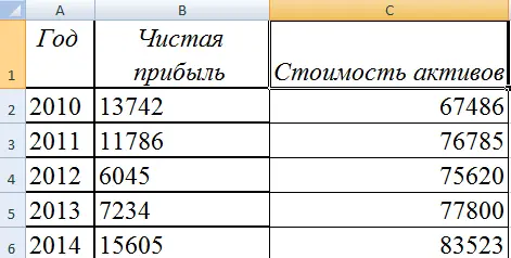
The main purpose of any graph is to show how values have changed over time. Let’s assume that we have such a table containing information about how much net profit was received by the organization in the last five years.
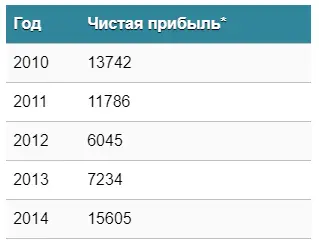
We provide these figures solely to demonstrate the operation of the graph. They do not correspond to any real company and are not tied to any currency.
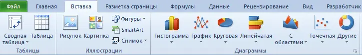
Next, we need to open the “Insert” tab, where you can select different types of charts. Let’s choose “Graph” as it fits our theme the most. At the same time, the logic is the same for all types of charts, so you can choose any other.
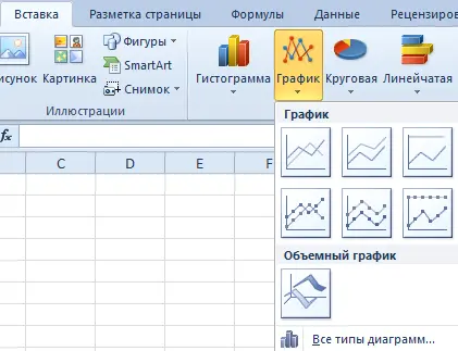
After we select the type of chart, a window will appear where you can select the type of chart. Excel also gives recommendations in which situations one or another option is better. To get a hint, just hover over it with the mouse cursor and wait a bit.
After the chart has been selected, it is necessary to set the source table in the chart area. As a result, we will get the following.
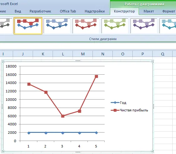
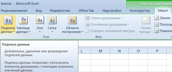
We see one defect. The blue line is completely useless in our example, so it should be removed. To do this, simply select it and press the Delete key. In the same way, the legend is removed, which is also not needed in our case (since there is only one curve). At the same time, it is desirable to sign the markers so that it is immediately clear what they mean. This opens the Data Labels tab.
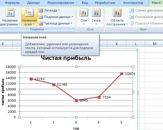
It is also desirable to sign the axes. To do this, you need to use the appropriate menu on the “Layout” tab.
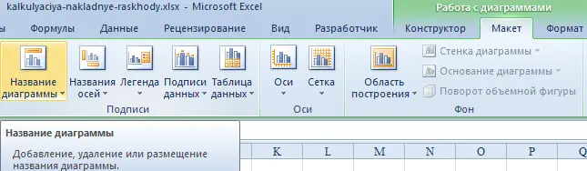
In the same way, the heading is removed if it is not needed. This is done by moving it outside the chart. You can also perform a number of other operations using the “Chart Name” item.
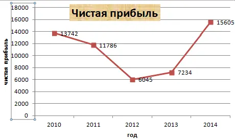
We use the year as the reporting year, and not its serial number, as originally suggested by the program. We should highlight the values of the axis where the time is displayed. After that, right-click and select “Select Data” – “Change Horizontal Axis Labels”. Next, a tab will appear where the data to be applied is selected. In our example, this is the first column.
The user has the opportunity to both leave the chart in its original form and format it. You can also move the chart to another sheet using the Design tab. That is where the option of the same name is located.
Creating a plot with two curves
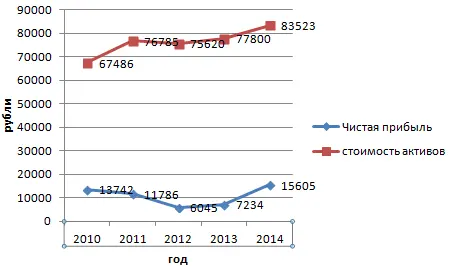
Suppose we are faced with the task of indicating not only the net profit of the enterprise, but also the total price of all assets in its account. There will be more information to display in the chart. Is it possible to create a chart that takes into account all these indicators without having to create another one?
Of course yes. Moreover, you do not need to perform fundamentally different actions. Only in this case, you do not need to remove the legend, since it denotes each of the axes, allowing the reader of the chart to understand what indicator each of them shows.
Inserting an additional axle
What actions should be taken if we want to add another axis? For example, it is useful if you use several different types of data or units of measure.
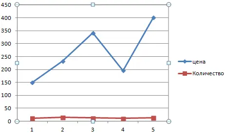
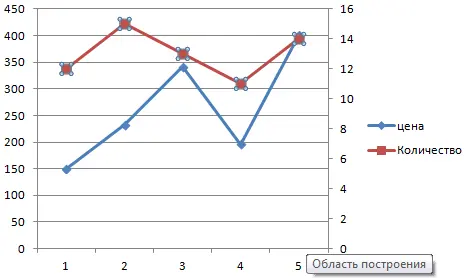
The first stage is similar to the previous one. It is necessary to build a graph in such a way, as if all of our data belongs to the same type.
After that, the axis to which the auxiliary one will be added is selected, right-click is made. Next, go to the options “Data Series Format” – “Series Parameters” – “Along the Auxiliary Axis”.
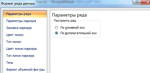
After we click the “Close” button, another axis will appear on the graph, which describes the information of the second curve (in our example, the one in blue).
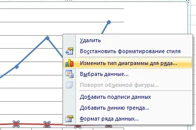
Also in the functionality of Excel there is another method – changing the type of chart. In this case, first a right click is made on the line to which the additional axis will be added. After that, a menu appears in front of us, in which we are interested in the option “Change chart type for a series.”
After that, we need to understand how the graph of the second data series will be displayed. In our case, we made a bar chart because it seemed to us that this way of presentation was the most convenient. But you have the opportunity to choose any other option.
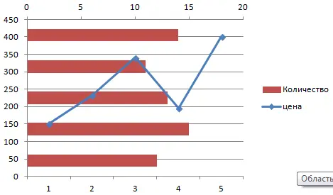
As you can see, it is enough to make only a few clicks to attach another axis to the chart, which describes measurements of a different type.
Plotting a Function
We all remember from school days what a function is. In algebra class, a very popular task was to plot a function graph. Excel gives you the opportunity to do this automatically in just two steps. First, a range with data is created, and then the chart is directly plotted.
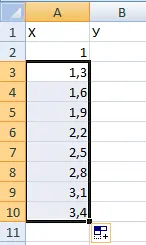
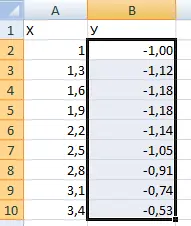
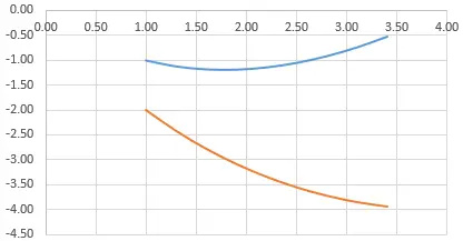
Suppose our function is: y=x(√x – 2). Step – 0,3.
Our first step is to create a function table with two columns. The first is X. To fill it in, you need to write 1 in the first cell and 1,3 in the second. You can use the formula =previous cell + 0,3. After that, you need to take the left mouse button on the lower right corner of the cell (it is in the form of a square called the autofill marker), after which it stretches down to the required number of cells.
The Y column in our example will be used to calculate the function. To do this, enter the formula in the first cell =A2*(ROOT(A2)-2) and press the “Enter” key. The value is calculated automatically. Further, the formula is multiplied throughout the column in a similar way to the previous one.
Everything, now the table with basic information is ready.
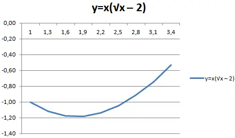
After that, we should understand on which sheet to insert the chart. This is done on both the new sheet and the existing sheet. In the first case, you need to create it. If the chart is inserted on the same sheet, then it is enough to select the required cell. Next, use the items “Insert” – “Diagram” – “Scatter”. A list of different chart types appears. We have the opportunity to choose the most suitable specifically for us.
Next, select the first column and click “Add”. After that, a window will pop up in which you need to set the name of the row using the function. The “X Values” field contains information from the first column. Accordingly, the range of the second column is written in the “Y Values” field.
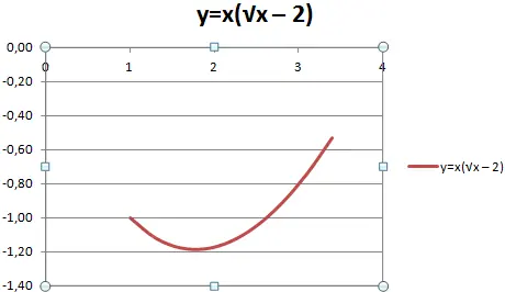
As you can see, the X axis does not contain values, while they are on the vertical one. Therefore, it is necessary to make the correct labels for the axes. Simply right-click on the X-axis, then click on “Select Data”, and then click on the item “Change Horizontal Axis Labels”. After that, we select the required range (in simple words, the table that contains the data we need), and then the graph takes on the correct form.
How to merge charts and overlay them on top of each other
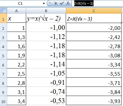
We see that it is not difficult to build two separate graphs, no matter how many axes are used there. But what if you need to combine two charts into one? Suppose we need to display two functions. One – the one that was before, and the other – which is shown in the table below.
After that, the necessary cells are selected and inserted into the chart. If it turns out that something did not go according to plan, you can correct the situation through the “Select Data” tab.
Dependency graphs in Excel – creation features
A dependency graph is a chart where the data in one column or row changes when the values in another are edited.
To create a dependency graph, you need to make such a plate.
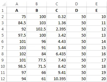
Conditions: A = f (E); B = f (E); C = f (E); D = f (E).
Next, you need to select the desired type. Here, let it be, according to the old tradition, dotted, as well as with smooth curves and markers.
After that, click on the “Data Selection” item, which is already familiar to us, and then click on “Add”. Values are inserted according to the following logic:
- For row name A, the horizontal values are A values. The vertical value is E.
- After that, the “Add” button is pressed again, after which for row B, values B are inserted as horizontal values, and the same value E is inserted vertically.
Thus, the entire table is processed. The result is such a cute dependency graph.
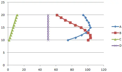
Chart Formatting
Here you can either stop or start editing the chart view. Formatting can be both simple and complex. Here we describe the basic functions.
As you can see, once the chart is selected, the Design and Format tabs automatically appear on the ribbon. With their help, you can customize the appearance of the charts.
Quick format
Excel provides a set of templates that allow you to quickly design any chart. They are called styles. Microsoft has provided 2 ways to define the chart style:
- Go to the “Designer” tab and find the “Chart Styles” item there. Don’t forget to highlight the chart first. You can preview how this or that diagram will look like. If you need to apply the desired style, just click on the appropriate option.
- Using the Chart Styles button that appears after selecting a chart. This method works in the same way as the previous one, but the styles are displayed not on the ribbon, but on the right pane.
There is no fundamental difference between these two methods, so you can choose the one that suits you best.
Adding and Formatting Chart Elements
When creating charts, you can add additional chart elements. In the “Designer” tab there is a button “Add Chart Elements”. After pressing it, a list of all elements appears. Just select the one you want and click.
You can also do the same through the “Chart Elements” button that appears after the chart is selected. After clicking it, a panel appears where you can configure the necessary elements with a checkmark. After that, we configure their location, and that’s it.
Most of the formatting options are found on the Format taskbar, which was first added by developers in Excel 2013. Previously, this was a normal dialog box. To open it, click on the chart and press Ctrl + 1. After that, double-click on the required element, then the context menu is called and the “Format” item is selected.
If the version of Excel is newer, then just find the Format Selected button on the Format tab, which is located on the ribbon, and click on it.
In any case, the “Format” window contains the same features, such as shading and borders, effects, parameters and sizes of different chart objects, color, and so on.
Conclusions
Thus, plotting in Excel is an easy task that does not require special skills. It allows you to present a huge set of data in an easy-to-understand way. This is useful in a variety of areas, from the educational process to the presentation of a business project to potential investors.