How to merge tables with partial match in Excel

This guide will describe what steps you need to take to quickly join data from two tables that do not have matches in key columns. That is, what to do if the identifier of one table matches only the first 5 values ​​of the identifier of the second table. All the methods that will be described today have been tested on Excel 2007 versions and others, up to the most modern ones.

Above are two documents. The first contains descriptions of the products sold by the company and their cost, and the second contains information about their availability in the warehouse. Each has its own unique identifier, which does not change regardless of how many times the “price” field or the “description” field is adjusted.

There may be problems if the second spreadsheet was submitted by a different department or company. In this case, the identifier format may be different. For example, only the first digits can be saved, and then a prefix can be added. The match is partial. Of course, a person can understand that these are essentially the same identifier, but a computer is not so smart. This makes it much more difficult to merge data from two files.

The situation can be aggravated by the fact that in one file the company may be called “Products”, and in another – “Products Corporation”. On top of that, you have one company signed as “New Organization” and another as “Old Company”. But it’s the same company. But only you know about it – but not a blind computer algorithm.

Note! The solutions described in this article can be used in absolutely any formula, such as VPR(), SEARCH(), GPR().

If you are not an Excel professional and do not want to complicate your life with additional instructions, you can use the add-on to merge data from two documents.

It is paid, but it allows you to quickly implement the task considered in this article. This is the only thing the add-on does, but it does it very well. Instead of writing long formulas, you just need to launch the virtual assistant and follow 5 steps to get the desired result. 

This addon can be used for 15 days, after which you need to pay for it. But the add-on is worth the money you pay for it, as it can save you a huge amount of time and nerves: about an hour to learn how to use the formulas. And in some cases – up to 20 hours, aimed at studying all the points and correcting all errors.

But for one-time use, the free version is enough.

If the id column contains additional characters

Let’s say you have two sheets. The first one contains the identifier, the name of the beer and its cost. The second contains the identifier and the number of bottles that are currently in stock. In life, any other product can be signed this way, and the numbers will be different.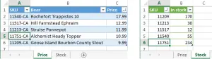

In the first table, the first column is a unique identifier, from which we need the first 5 characters. We add an additional column to the right one called “SKU helper”. Next, you need to follow this instruction:

1. Place the mouse cursor next to the column name. It will become like an arrow, as shown in the screenshot.
2. Right-click on it to bring up the context menu, and then select “Paste”.
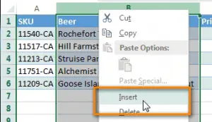
3. Name the column “SKU helper”.
4. To get the first five characters from the SKU column, you need to find the required cell in the newly formed column and enter the formula =LEFT(A2). In the described case, A2 is a reference to the cell to be searched, and the second argument is the number of characters that the program should extract.
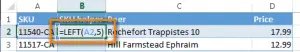
5. Further, this function is copied to all other cells by dragging the cell located in the lower right corner to as many lines as necessary. Or you can selectively copy it in the standard way (using the key combination Ctrl + C – Ctrl + V).

It’s all! Now you have a ready-made column whose values ​​correspond exactly to the contents of another table. Data will be searched in the SKU column, and the result will be displayed in the SKU helper. And finally, you need to use the function VPR to get the required result.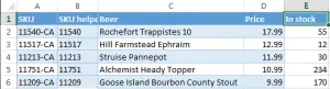

What other formulas can be used?

1. To extract a certain number of characters from the right, you need to use the function =RIGHT. The syntax is similar. For example, the formula would look like this: =RIGHT(A2). 
2. You can use the formula =PSTR, to extract a certain combination of characters from the middle. For example, you can skip the first 8 characters and extract the next 4. As a result, the formula will look something like this.  =MID(A2)
3. You can get all the characters that are up to a certain sign. The number of digits that will be copied may differ. For example, a program might extract 233 and 34 from the values ​​”233-pp” and “34-pp” respectively. To do this, you need to modify the =LEFT formula by adding the “FIND” formula to the argument. 

Thus, to find parts of the index, you can use the formulas “LEFT”, “RIGHT”, “MID”, “FIND”. 

If the information in the key column of the first document is divided into several columns in another

For example, in the first table there is a main column with ID. The cell describes values ​​of the form XXXX-YYYY, where XXXX is the identifier of the product group, and YYYY is the code of the specific product in this group. We do not have the ability to ignore the belonging of a product to a certain group, since the same identifier can be in products of different categories.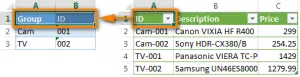

To do this, you need to add an additional column, naming it “Full ID” as described above. In our example, it should be in column C. Next, you need to use the formula =CONCATENATE in cell C2. The function has three arguments:

1. The address of the first cell.
2. Separator.
3. The address of the second cell.

It looks like this:

=CONCATENATE(A2;”-“;B2)

After this formula is entered in the first cell of the column, it must be copied to the bottom of the column.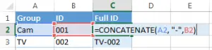

Now you can easily combine data from multiple spreadsheets. We compare the “Full ID” column with the “ID” column of the table we are looking for. If the parameters match, we add entries from the description and price columns that are in the desired table.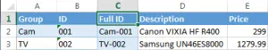

If the data in different key columns does not match at all

Let’s say you have a small store and you get products from one or more suppliers. Each of them identifies the goods in their own way. Therefore, it may be that a product encoded by the “Case-Ip4S-01” entry in the supplier’s document will be encoded as “SPK-A1403”. Moreover, there is no logic by which you can set a rule for automatically converting an identifier from one format to another.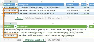

The bad thing here is that all the data will have to be processed manually. But in the future, you can automate this process if you process the document once. To do this, follow these instructions:

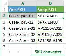
1. Create a new document with the name “SKU converter” or any other name. Next, you need to copy the Our.SKU column to a new sheet, and also remove all duplicate parts of the values.
2. After that, the Supp.SKU column is added and manually matched between your columns and the manufacturer ID column.
3. The result will be the same as in the screenshot.
4. This table should now be updated with the information provided in the search sheet.

After that, the second stage begins, during which the following actions are performed:

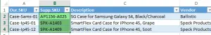
1. After the first column, the Supp.SKU column is inserted.
2. Next, the VLOOKUP function is used, with the help of which the Store and SKU converter sheets are compared. Matches are looked up in the Our.SKU column, and the updated data will be stored in the Supp.SKU column. If, after applying the formula, some cells remain empty, you should take all the SKU codes that correspond to these cells, add them to the SKU converter table, and then find the required code in the supplier table. After that, this step is repeated.
3. Information from the lookup table is transferred to the main one, where there is a key column with the corresponding elements of the lookup table.

The result is a table like this.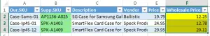

Tell me, it’s simple, right? The main thing is to get used to it a little. Of course, the last case is the most difficult, but even here you can partially automate the process.

If you don’t want to deal with all the moments of combining tables with different data, you can use the above addition to the standard Excel package. Although it is commercial, but the first days it can be used for free. If there is no need to constantly merge tables with different data, then there is no point in learning this bunch of formulas. It is enough to use the add-on once. And if you need to merge tables regularly, this addon can save you a lot of time.