


Contents
Strikethrough text is a great way to show that some data is out of date. In particular, formatting text in this way is often necessary in Excel. For example, you can change the text formatting when a certain condition is met. Or to carry out strikethrough of the text in the manual mode.
When a user wants to try this feature for the first time, they may not succeed. The fact is that strikethrough text in Excel is far from the most intuitive procedure. But still, let’s figure out what needs to be done in order to make a strikethrough text in Excel.
What is the purpose of crossed out text in Excel
There are many uses for strikethrough text. As mentioned earlier, this may be an emphasis on the irrelevance of some information. Strikethrough text can also be used in the following cases:
- To indicate the changes to be made.
- as an artistic medium. Sometimes this is how the hidden meaning of the sentence is shown in the text, where the first few words are crossed out. They are just the hidden meaning of the sentence. For example, “I would never want to see you My work load has suddenly increased, and I can’t meet.” Sometimes this formatting needs to be applied in Excel as well. For example, list practical examples of metacommunications in tabular form.
As well as many other applications, the ideas of which may arise spontaneously. Let’s now proceed directly to how to implement text strikethrough.
How to strikethrough text in excel
Since strikethrough is a formatting element, the user can use specialized tools to implement this feature. Let’s look at them in more detail.
This method has become very popular among Excel users because it is one of the most intuitive of all. Anyone who has used Excel a little can find it. But so that you do not waste time, we will teach you how to do it as quickly as possible. Do the following sequence of actions:
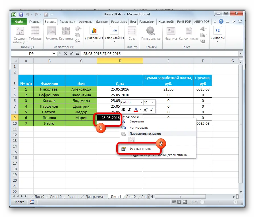
- Select the cell or the set of cells that you want to use to make formatting settings. Then do the right mouse click. After that, a menu called context menu will appear. It gets its name from the fact that its content always depends on the scope from which it is called. Therefore, if we select a cell and right-click on it, the cell settings menu will appear. In this list, we are interested in the item “Cell Format”, on which you need to click.
- After that, the cell formatting settings window will appear. In it we find the tab “Font”, go through it and select the item “Strikethrough”. To do this, you must check the appropriate box. After that, we confirm our actions (that is, we press the “OK” button).


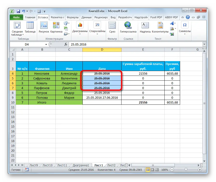
- After we completed these steps, all the letters turned out to be crossed out. Our goal has been reached.

Format individual words in cells
Often, only certain words in a cell need to be crossed out. In this case, the sequence of actions will be somewhat different:
- First, double-click on the part of the cell that we want to cross out. After that, we have a text input field. We need to select the area that needs to be crossed out.
- We call the context menu with a single right-click, as in the previous example. We see that since our context has changed, the appearance of the context menu will also change. Nevertheless, there you need to select the same item as in the previous method – “Format cells …”.

- We see that the window itself has a different look. Now there is only one tab where we need to find the “Strikethrough” item and check the box next to it. After that, we confirm our actions again by clicking on “OK”.


Now we check the result and see that our attempt to strike out only part of the text in the cell was successful. 
Through the tools on the ribbon
Few people know that you can also find tools on the ribbon that allow you to make strikethrough text. To do this, we perform the following sequence of steps:
- We highlight the information that we need to cross out. It can be either the cell itself, or the range, or the text inside. After that, open the “Home” tab. Next, we find the “Font” group and open it by clicking on a special icon in the lower right corner.

- After that, a settings window will open, which differs depending on what information was selected in the first step. But the tab will open correctly, even if it has full functionality. Further, the sequence of actions is the same as in the previous methods: you need to check the box next to the “crossed out” item and press the “OK” key.

Applying a keyboard shortcut
The least intuitive way, but also the easiest and fastest once you learn about it. It is necessary to select a cell, a range or a separate text and press the hot keys Ctrl + 5.

While this method is indeed much more convenient than the previous ones, it can be quite tricky for beginners as they have to keep a lot of keyboard shortcuts in mind.
Conclusion
All described methods have an equal right to exist. Depending on the goal that the user sets for himself, you need to use a different method. The most universal is the use of a combination of hot keys, but it also has its limitations. If a person encounters them for the first time, it can be quite difficult for him to remember the correct sequence of characters, especially since there is no logic in it, unlike Ctrl + C, where it is clear that C stands for the word Copy (copy).
In any case, with practice, all hotkeys are brought to automatism, so the more often you use this combination, the easier it will be to remember. Therefore, it is recommended that you definitely practice before using these methods.