


Contents
If an Excel user has to work with a large table and is faced with the task of finding unique values that fall under a certain criterion, then he often has to use a tool such as a filter. But in some cases it is necessary to do something else, namely, to select all the series in which there are certain values in relation to other series. If we talk about this situation, then here you need to use another function – conditional formatting.
To maximize the return, you need to use a drop-down list as a request.
This is well suited for situations where you need to keep changing queries of the same type to expose different rows in a range. Now we will describe in detail what actions must be performed in order to create a selection from the repeating cells that are part of the drop-down list.
How to select unique and duplicate values in Excel – step by step instructions
First of all, we need to understand what a sample is. This is one of the most important statistical concepts, which means a set of parameters selected according to a certain criterion. Anything can act as a sample: people for the experiment, clothes, enterprises, securities, and so on.
To create a sample, you must first select those results that fit the conditions from a large list, and then display these values in a separate list or in the original table.
Preparing the contents of the dropdown list
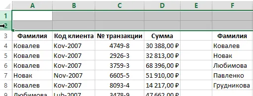
To make our work today more visual, let’s take the history of settlements with customers. It will look like the picture. 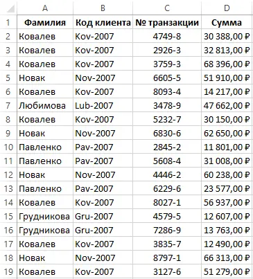
Here we need to highlight all the operations performed in relation to each specific counterparty using color. To switch between them, use the dropdown list. Therefore, initially you need to make it, and for this you need to select the data that will be its elements. In our example, we need all the names of counterparties that are in column A and are not repeated. To prepare the contents of the dropdown list, we need to execute the following statement:
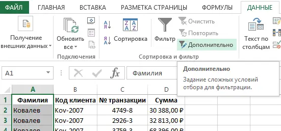
- Select the first column of our table.
- Use the tool “Data” – “Sort and Filter” – “Advanced”.

- After that, a window will appear in front of us, in which we need to select the type of processing “copy the result to another location”, and also check the box next to the item “Only unique records”. In our case, the range we are using will be the cell with the address $F$1. The dollar sign means that the link is absolute and will not change depending on whether a person copies or pastes the contents of the cell that is linked to it.
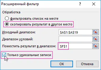

- After we set all the necessary parameters, we need to press the OK button and so we confirm our actions.
Now we see a list of cells with unique surnames that are no longer repeated. This will be our selection for the list. 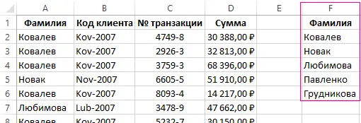
Modification of the original table
After that, we need to make some changes to our table. To do this, select the first two rows and press the key combination Ctrl+Shift+=. Thus, we insert two additional lines. In the newly created cell A1, insert the word “Client”.
Create a dropdown list
After that, we need to create a dropdown list. To do this, follow these steps:
- Click on cell B1. Go to the tab “Data” – “Working with data” – “Data validation”.


- A dialog box will appear in which we need to select the “List” data type, and select our list of surnames as a data source. After that, click on the OK button.
After that, cell B1 turns into a complete list of customer names. If the information that serves as the source for the drop-down list is located on another sheet, then in this case it is better to make this range named and refer to it in this way.
In the case of us, there is no need for this, because we already have all the information on one sheet.
Selecting cells from a table by condition
Now let’s try to create a selection of cells by condition. To do this, select the table that contains the name of the counterparty, its code, transaction number and transaction amount, after which we will open the “Conditional Formatting” window. To call it, you need to go to the “Home” tab, find the “Styles” group there, and there will be a “Conditional Formatting” button in it.
A menu will appear in which we need to click on the “Create Rule” item, for which we select “Use a formula to determine formatted cells.” 
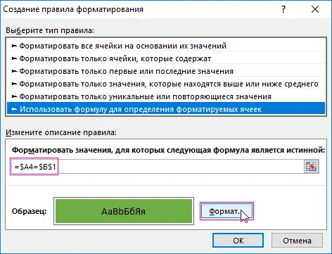
Next, enter the formula shown in the screenshot, and then click on the “Format” button to make all cells containing the same last name a color. For example, green. After that, we confirm all the actions performed earlier by repeatedly clicking on “OK” on all windows that will be open at that time. After that, when we select the last name of our person, all cells that include it are highlighted in the color that we set.
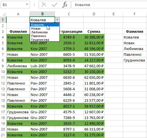
How it works? When we select a value in the drop-down list, the formula analyzes all available rows, and if it sees a match, it highlights them in a user-defined color. You can verify that the formula works by choosing a different surname. After that, the selection will change. This makes the table much easier to read.
The principle of operation is as follows: the value in column A is checked. If it is equal to the one selected in the list located in cell B1, then this formula returns the value TRUE. After that, the whole line is formatted the way you want. In principle, you can not only highlight this line with a separate color, but also arbitrarily adjust the font, borders and other parameters. But highlighting is the fastest method.
How did we achieve that the whole line is colored with color, and not a separate cell? To do this, we used a cell reference, where the column address is absolute and the row number is relative.
Download an example of selecting from a list with conditional formatting
How it works? You can try to look visually by downloading an example of such a table, which we reviewed earlier. To do this, follow this link.
4 ways to select data in Excel
But this is not the end of our guide. In fact, we have as many as four available ways to select data in Excel.
Advanced AutoFilter
This is the easiest method that allows you to select values that fit certain criteria. Let’s take a closer look at what is needed for this.
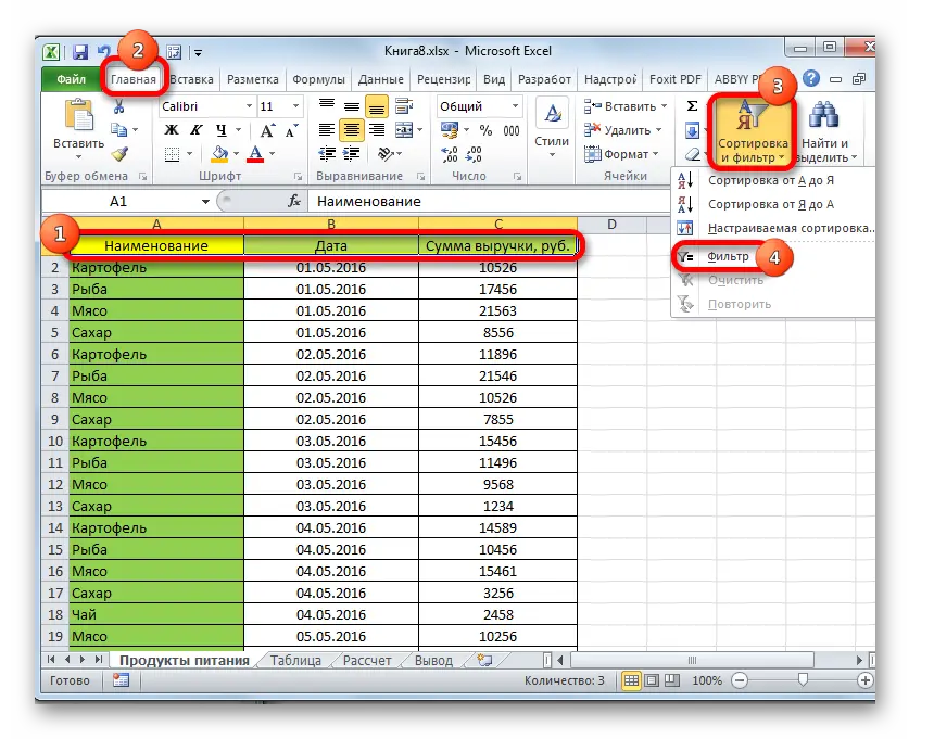
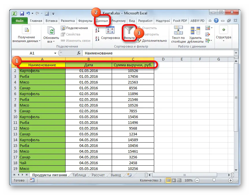
- Suppose we have a table containing the name of the product, the date and the total amount of money that was earned by selling a particular item on a particular day. We need to select the area where we need to select a sample. To do this, go to the “Home” tab, where we find the “Sort and Filter” button and click on it. It can be found in the “Editing” toolbox. After that, we find the option “Filter”. We provide a screenshot for clarity.

- There is another way to do this in this case. You can find the Filter button in the Sort & Filter group on the Data tab.

- After we do this, arrows will appear at the top of the table, with which you can select data for the filter. You need to click on one of them (which one depends on the column in which we need to sort). After that, we find the item “Numeric filters”, and click on “Custom filter”.
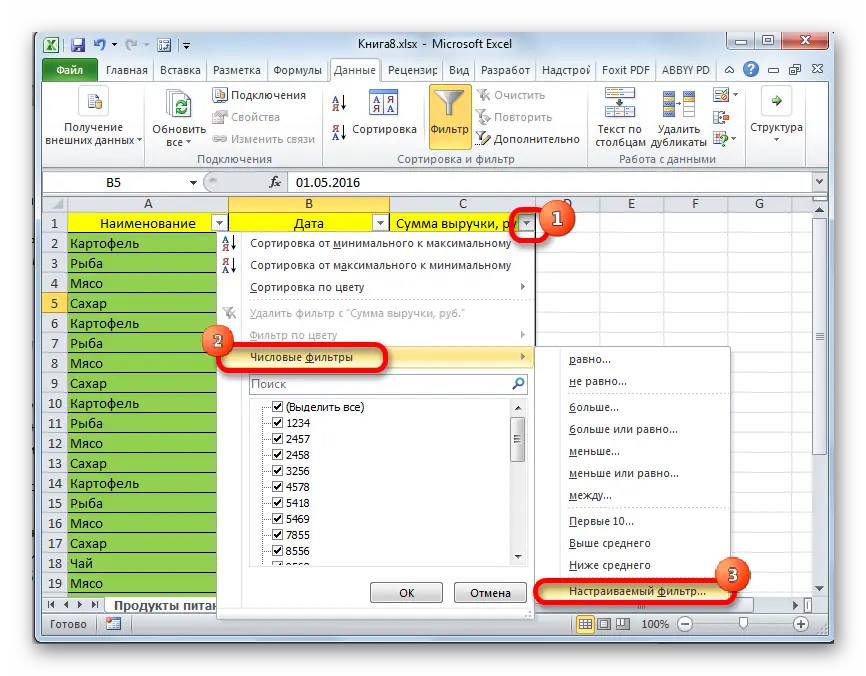

- After that, a window appears through which you can configure custom filtering. With it, the user can set the criteria based on which the data will be selected. In the drop-down list for the column that contains numeric cells (namely, we use them for example), it is possible to select criteria such as equal, not equal, greater than, greater than or equal to and less than. That is, standard arithmetic comparison operations.
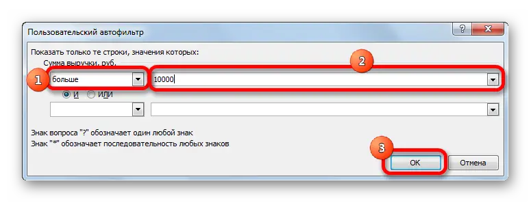
For clarity, let’s set a rule according to which the program should select only those values in which the amount of revenue is more than 10 thousand rubles. Therefore, we need to set the “more” item in the field marked with the number 1 in the screenshot, and set the value of 2 thousand (in numbers) in the field marked with the number 10. Next, it remains only to confirm our actions.

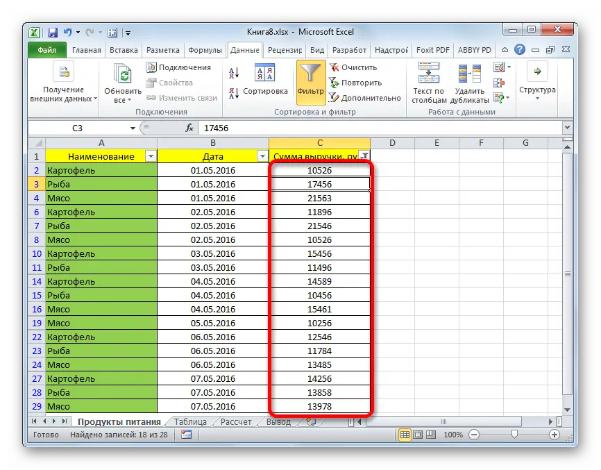
- As we understand, after we filtered the data, only those lines remained in which the amount of money earned without deducting taxes is more than 10 thousand rubles.
- But we have the opportunity to add one more criterion. To do this, we must again return to the custom filter, at the bottom of which we see two more fields that have the same form as the one in which we entered our criteria. You can set the second parameter in it. Let, for example, we need to select only those data that do not exceed 14999. To do this, select the “Less than” rule, and set the value to “15000”.
You can also use the condition switch, which can take one of two values: AND and OR. Initially, it is set to the first option, but if a person needs to match one of these conditions, then the OR value can be selected. To switch the type of relationship between conditions, you must put the toggle switch in the appropriate position. After we have completed all the necessary steps, click on the “OK” button.
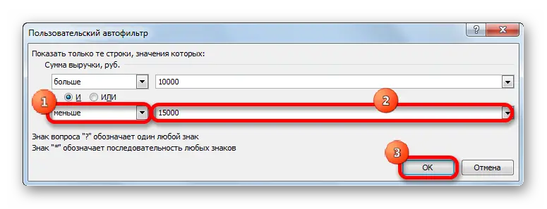

- Now our table displays only those values that range from 10 thousand rubles to 14999 rubles.
Array Formula
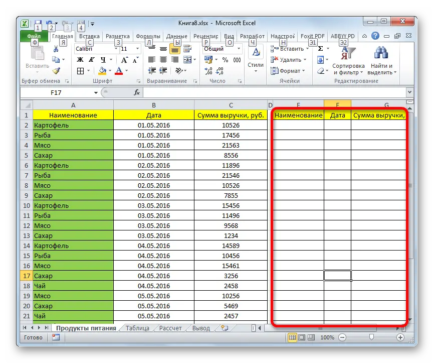
Another selection option is to use an array formula. In this case, the result is displayed in a separate table, which can be useful if you always need to have the original data in front of your eyes unchanged. To do this, we need the following:
- Copy the table header to the desired location.

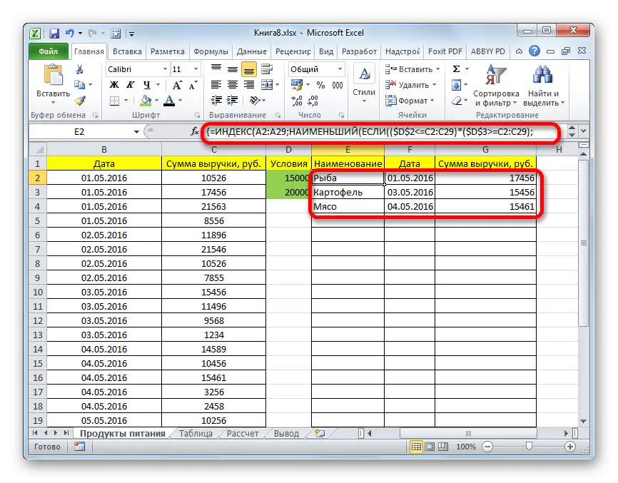
- Select all the cells that are contained in the first column of the newly created table and move the cursor to the formula input line. After that, we insert the following formula there (we change the values, of course, to our own). =ИНДЕКС(A2:A29;НАИМЕНЬШИЙ(ЕСЛИ(15000
- Confirm the input using the key combination Ctrl + Shift + Enter.
- We perform a similar operation with the second column.
- We do the same with the third column.
In all three situations, the formula is basically the same, just the coordinates change.
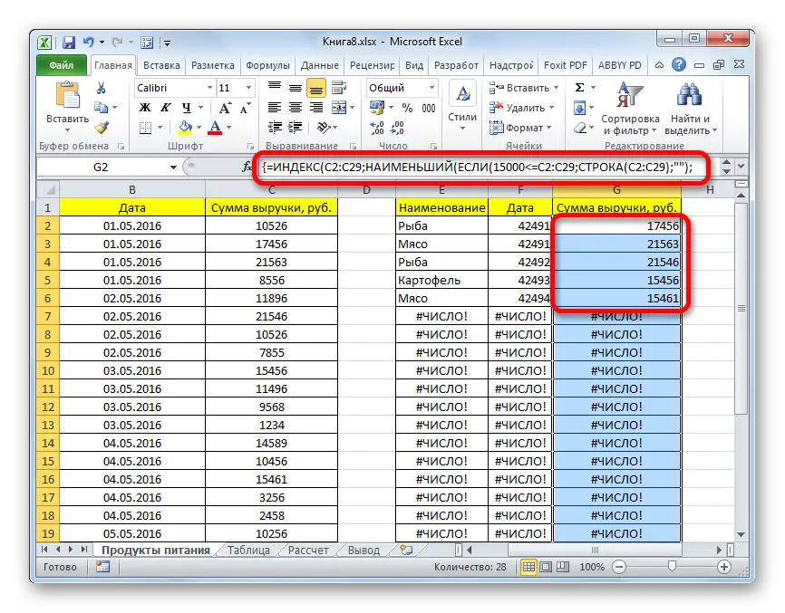
After that, we assign the correct format to the cells in which the error appears. Next, we use conditional formatting to highlight those cells that contain a specific value.
Selecting with multiple conditions using a formula
Using formulas also allows you to select values based on multiple criteria. To do this, perform the following steps:
- We set the conditions in a special column of the table.
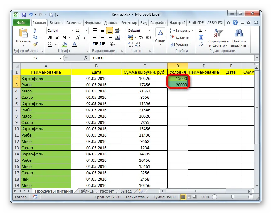
- We write three formulas with the correct coordinates in each of the auxiliary columns that must first be created. In the same way, we use an array formula for this.
The advantage of this method is that there is no need to change the formula if you suddenly need to change the conditions. They will always be stored in their respective cells.
random sample
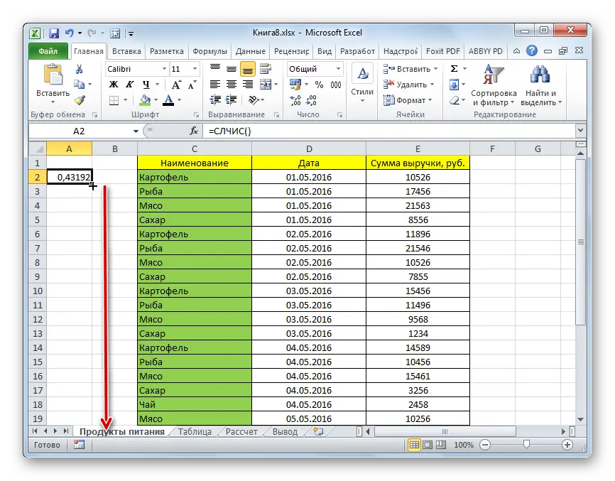
And finally, the last sampling method, which is not suitable in all situations, is the use of a random number generator. To do this, you need to use the function =SUM(). Next, we fill in as many cells as we need using the autofill marker.
Next, select “Custom Sort” from the filter menu.
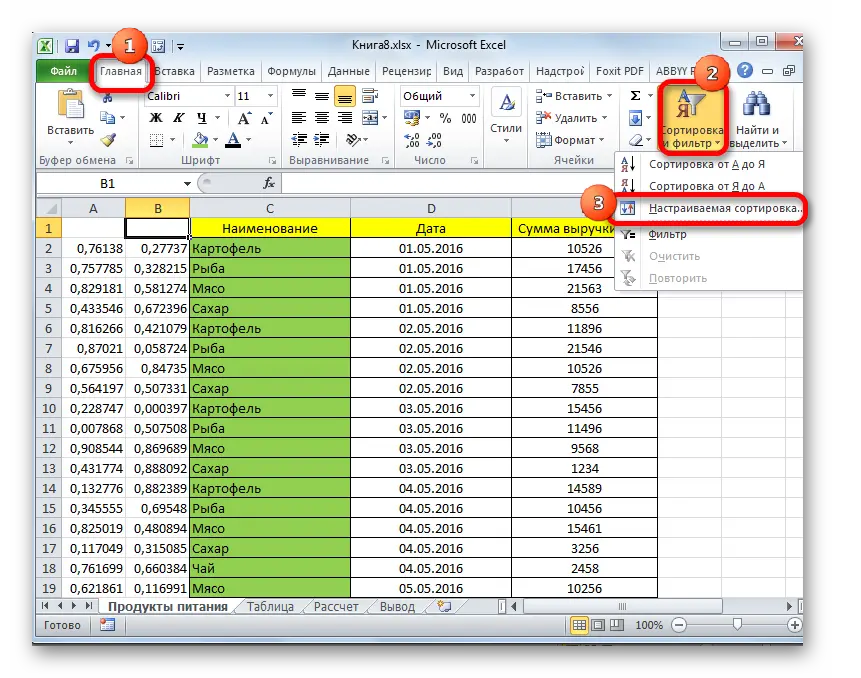
The settings menu appears, where we set the parameters as in the screenshot. 
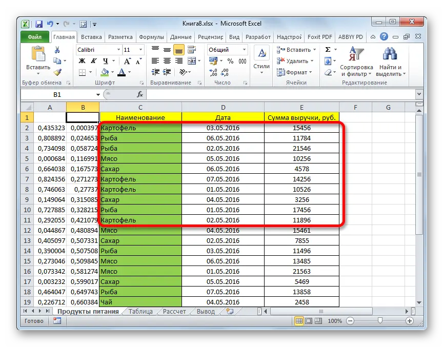
Then click “OK” and get the result.
We see that there is nothing complicated. With a little practice, everything will turn out very easily. The main thing is to understand the principle, and you can choose any method you like.