


Conditional formatting in Excel allows you to change the format of cells depending on their content. For example, you can force a cell to change color if it contains a value less than 100, or if that cell contains certain text. But how to make it so that not only one cell becomes selected, but the entire line that contains it?
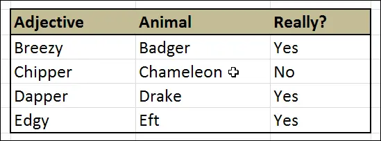
What if you need to select other cells depending on the value of one? In the screenshot above, you can see a table with the code names of various versions of Ubuntu. One of them is fictional. When I entered No in a column Really?, the entire row has changed background and font color. Read on and you’ll find out how it’s done.
Create a table
First of all, we create a simple table and fill it with data. Later we will format this data. Data can be of any type: text, numbers, or formulas. At this stage, the table has no formatting at all:

Making the table look nicer
The next step is to make the table format easier to read using Excel’s simple formatting tools. Adjust the format of only those areas of the table that will not be affected by conditional formatting. In our case, we will draw the frame of the table and format the row containing the headings. I think you can handle this part on your own. In the end, you should end up with something like this (or maybe a little prettier):
Create Conditional Formatting Rules in Excel
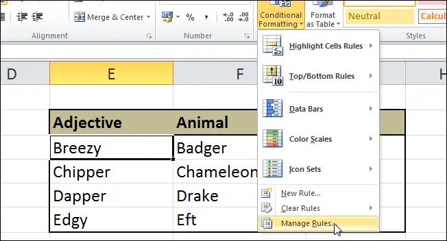
Select the starting cell in the first of the rows you plan to format. Click Conditional Formatting (Conditional Formatting) tab Home (Home) and select Manage Rules (Rules Management).
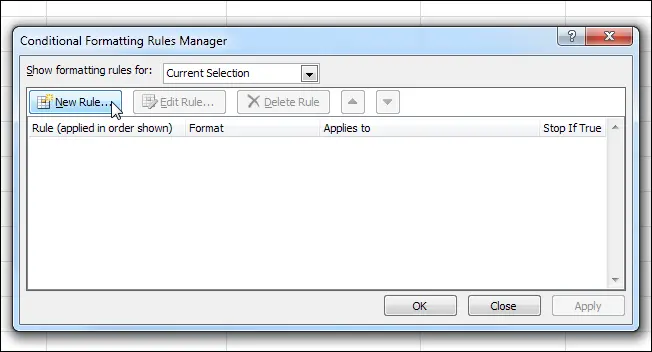
In the opened dialog box Conditional Formatting Rules Manager (Conditional Formatting Rules Manager) click New Rules (Create a rule).
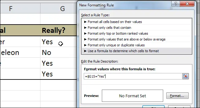
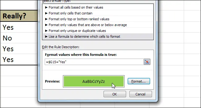
In the dialog box New Formatting Rule (Create Formatting Rule) select the last option from the list − Use a formula to determine which cells to format (Use a formula to determine which cells to format). And now – the main secret! Your formula should return a value TRUE CODE (TRUE) for the rule to work, and must be flexible enough that you can use the same formula to work with your spreadsheet.
Let’s analyze the formula I made in my example:
=$G15 is the address of the cell.
G is the column that controls how the rule works (column Really? in the table). Notice the dollar sign in front of the G? If you do not put this symbol and copy the rule to the next cell, then the cell address in the rule will shift. So the rule will look for the value Yes, in some other cell, for example, H15 instead G15. In our case, we need to fix the column reference ($G) in the formula, while allowing row (15) to change, since we are going to apply this rule for several rows.
=»Yes» is the cell value we are looking for. In our case, the condition cannot be easier to imagine, the cell should say Yes. You can create any conditions that your imagination tells you!
In human terms, the expression written in our formula takes on the value TRUE CODE (TRUE) if the cell located at the intersection of the given row and column G contains the word Yes.
Now let’s do some formatting. Click the button Size (Format). In the opened window Format Cells (Cell Format) scroll through the tabs and adjust all the settings as you wish. In our example, we will simply change the background color of the cells.
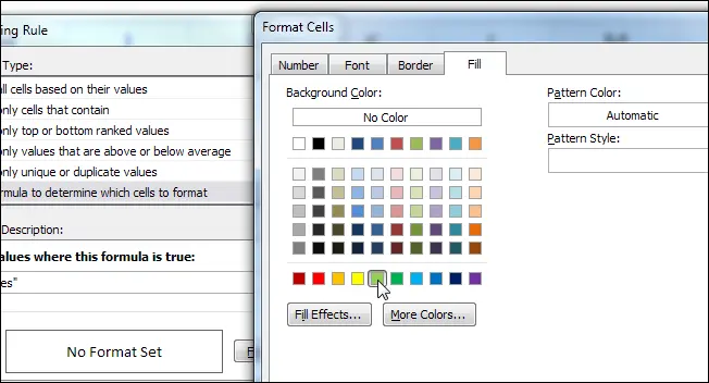
When you have set the desired cell appearance, click OK. You can see how the formatted cell will look in the window Preview (Sample) dialog box New Formatting Rule (Create a formatting rule).
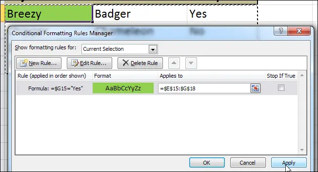
Press OK again to return to the dialog Conditional Formatting Rules Manager (Conditional Formatting Rules Manager), and click Apply (Apply). If the selected cell has changed its format, then your formula is correct. If the formatting hasn’t changed, go back a few steps and check your formula settings.
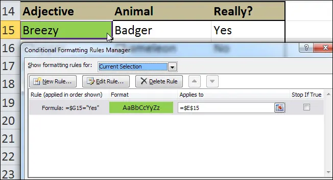
Now that we have a working formula in one cell, let’s apply it to the entire table. As you can see, the formatting has changed only in the cell we started with. Click on the icon to the right of the field Applies to (Applies to) to minimize the dialog box, and by clicking the left mouse button, drag a selection across your entire table.
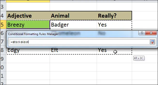
When done, click the icon to the right of the address field to return to the dialog box. The area you selected should remain dotted, and in the box Applies to (Applies to) now contains the address of a whole range rather than a single cell. Click Apply (Apply).
Now the format of each row of your table should change according to the created rule.
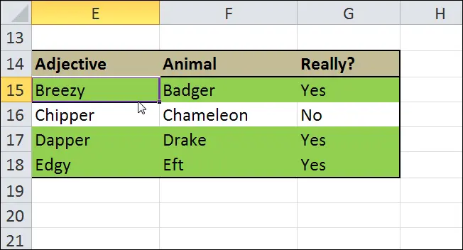
That’s all! Now it remains to create a formatting rule in the same way for rows that contain a cell with a value No (because a version of Ubuntu codenamed Chipper Chameleon never actually existed). If the data in your table is more complex than in this example, then you will probably need to create more rules. Using this method, you will easily create complex visual tables, the information in which is literally striking.