


Contents
In one of the previous articles, we successfully coped with the task and learned how to print grid lines on a paper page. Today I want to deal with another issue, also related to the grid. In this article, you will learn how to display the grid on the entire Excel sheet or only for selected cells, as well as how to hide lines by changing the fill color or cell border color.
When you open an Excel document, you see faint horizontal and vertical lines that divide the worksheet into cells. They are called grid lines. It is very convenient to have a grid visible on an Excel sheet, as the main idea of the application is to distribute data into rows and columns. There is no need to additionally draw cell borders to make the data table more understandable.
In Excel, the grid is displayed by default, but sometimes there are sheets where it is hidden. In such a situation, it may be necessary to make it visible again. It is also often necessary to hide the grid. If you think your worksheet will look neater and nicer without the grid lines, you can always make them invisible.
Whether you want to show the grid or, conversely, hide it, read this article carefully to the end and find out the different ways to perform these tasks in Excel 2010 and 2013.
Show grid in Excel
Suppose the grid is hidden and you want to make it visible on the entire worksheet or the entire workbook. In this case, you can configure the desired options on the Ribbon in Excel 2010 and 2013 in two ways.
First of all, open the sheet on which the grid is hidden.
Tip: If you need to show the grid on two or more Excel sheets, click on the tabs of the desired sheets at the bottom of the Excel window, while holding down the key Ctrl. Now any changes will be reflected in all selected sheets.
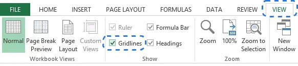
When the sheets are selected, open the tab View (View) and in section Show (Show) check the box next to Сетка (Gridlines).
Another way: on the tab Page layout (Page Layout) in the section Sheet options (Sheet Options) under the heading Сетка (Gridlines) check the box Show (View).
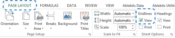
Whichever option you choose, the grid will immediately appear on the selected sheets.
Tip: To hide the grid on the sheet, just uncheck the options Сетка (Gridlines) or Show (View).
Show/hide the grid in Excel by changing the fill color
Another way to show/hide the grid in an Excel sheet is to use the tool Fill color (Fill Color). Excel hides the grid when cells have a white background color. If there is no fill in the cells, the grid will be visible. This technique can be applied to the entire sheet or to a selected range. Let’s see how it works.
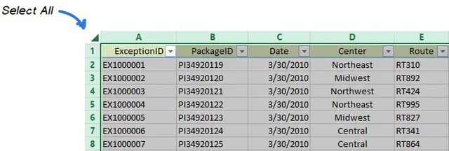
- Select the desired range or the entire sheet.
Tip: The easiest way to select an entire sheet is to click on the gray triangle in the upper left corner of the sheet at the intersection of the row and column headings.
 You can use the keyboard shortcut to select all cells on a sheet. Ctrl + A. If one of the cells in the Excel table is currently selected, then press Ctrl + A needed twice or thrice.
- On the Advanced tab Home (Home) section Font (Font) click on the dropdown list Fill color (Fill Color).
- To hide the grid, you need to select white cell fill color.
Tip: To show the grid in an Excel sheet, you need to select the option No fill (No Fill).
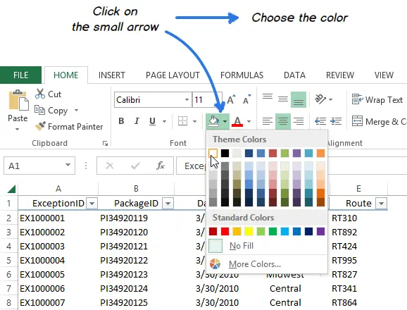
As shown in the image above, the white shading of the worksheet cells creates the effect of a hidden grid.
Hide grid lines in selected cells in Excel
If in Excel you need to hide the grid only in a certain limited range of cells, then you can use white fill or white color for cell borders. Since we have already tried changing the fill color, we will try to hide the grid by changing the border color of the cells.
- Select the range in which you want to remove the grid.
- Right-click on it and select from the context menu Cell format (Format Cells).
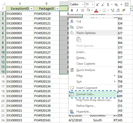
Tip: Dialog window Cell format (Format Cells) can also be called by pressing a keyboard shortcut Ctrl + 1.
- Open the tab Border (Border).
- Choose white color and under the heading All (Presets) press External (Outline) and internal (Inside).
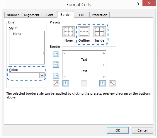
- Click here OKto see the result.
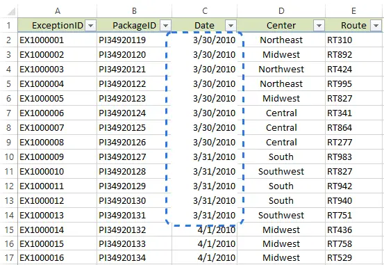
Ready! Now an area has appeared on the Excel sheet, which differs from the others in the absence of cell borders.
Tip: To show the grid again for the cells you just changed, open the dialog box Cell format (Format Cells) and on the tab Border (Border) under header All (Presets) click No (None).
Hide the grid by changing the color of its lines
There is another way to hide gridlines in Excel. To make the grid invisible on the entire worksheet, you can change its default line color to white. Those who wish to learn in detail how this is done will be interested in the article How to change the default grid line color and enable grid printing in Excel 2010/2013.
As you can see, there are various ways to hide and show gridlines in Excel. Choose the most suitable one for you. If you know other ways to hide or show the grid in Excel, share them in the comments. We will be very grateful to you!