


Contents
Very often, an Excel user has to work with tables that have a huge amount of information. For example, information about the salaries of employees of a large company. And often there is a situation when you need to compare the information in the cells with the table header. For example, to see how much salaries differ within the same company for electricians of the first category. Or directors of the enterprise and electricians. Not so important, the tasks in the work can be any, even the most bizarre.
And if the amount of data is very large, then the table is located very high, and constantly scrolling through the table in order to find it is very inconvenient.
But fixing a row or column in such situations can be a very correct way out of them. At the same time, no matter how much you go down the table, the top line will still be displayed on the screen. What to do to make it?
How to freeze a row in Excel on scroll
This is an absolutely easy task. Moreover, it is possible to display at the top not only one line, but also several. After work, you may need to remove the fastening of the line. We will look at methods on how to implement all these tasks.
In this case, the sequence of actions is slightly different depending on the version of Excel. So let’s look at an example of using this feature in newer versions and older versions (starting with Excel 2007).
How to freeze more than one row in a table
Sometimes it may be necessary to pin several lines at the top at once. For example, if you need to compare not only with the headings, but also with the first values of the corresponding columns. In the case of the above example about electricians, this could be a task to compare the salaries of specialists of the same skill level with the salary of the first in the list. In this case, the actions will be different from fixing just one line.
First you need to click on the leftmost cell, which is located under the rows that you want to fix. Let’s give an example in which cell A8 is such.
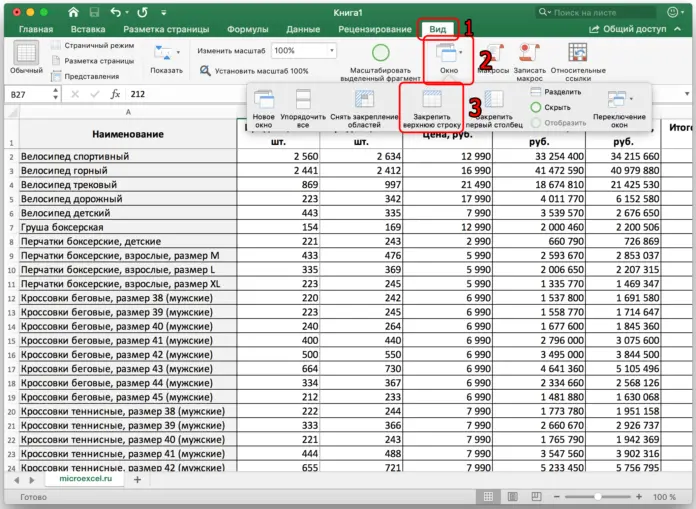
After that, you need to find the “View” tab, open it by pressing the left mouse button, and among the heaps of settings you need to find the “Window” button. A menu will appear in which you need to press the third button from the left. This is the function of pinning regions. Everything is simple.
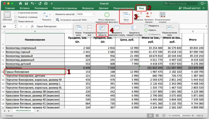
You can now scroll down any number of lines, because all lines above cell A7 will stay at the top.
The sequence of actions in Excel 2007 and other older versions is somewhat different. To do this, you need to follow these steps:
- Create a table and find data to fill it with. Well, write them down, of course.

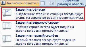
5 - After that, we click on the first left cell located under the line that needs to be fixed. Again, go to the “View” tab, as in the example with newer versions. In this case, the “Lock areas” button is located directly on the ribbon. You don’t need to click the Window button to do this. After pressing it, a list of functions will appear. In our case, we are interested in the “Lock areas” option.

6
After performing these actions, we will have fixed the number of rows above the cell on which the click was made. Thus, you can fix any number of cells that fit on the screen.
In fixed cells, you can perform all the operations that can be performed in normal cells. They will just always be at the top. That is, if you need to suddenly enter a formula that calculates the average value of numbers in a fixed range, it will be possible to do this.
In even older versions of the program, this tool can be found under the Window menu. A very large number of people still use the 2003 version, because their workplaces have not yet received new computers. It’s sad, but in general, the functionality of old Excel does not fundamentally differ from the new ones. Almost all basic functions, including freezing rows and columns, are preserved. And the logic does not change depending on the version.
How to fix the top row
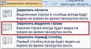
The mechanism of action is similar to the previous one. In the same way, you need to go to the “View” tab, in which you need to find the same “Window” button. The only difference is that we need to find the “Lock Top Row” option. If you look at the ribbon, the user will be able to find it directly to the right of the button we need. That is, in this situation, you need to click on the fourth button on the left in the menu that appears.
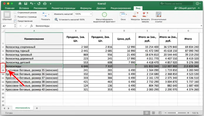
As you can see, the sequence of user actions is absolutely simple to understand. You can check yourself. We will do the same. As you can see, regardless of the number of rows that the table scrolls down, the row still remains in the visibility zone. In the screenshot, this can be seen in the red squares. Without fixing, the nineteenth line should have been preceded by the eighteenth. And we easily notice that instead of it we have row number 1. Thus, we can not get confused in the numbers and always understand which cell means what.
It is recommended that you test this feature before using it in a real environment. This will help you feel more confident.
To fix the top row in earlier versions of Excel while scrolling, you need to do almost the same steps: create a table, specify data. After that, click on “Freeze areas”, and there will be a function “Freeze the top row”. Here you can click absolutely on any cell of the table, not only the one that is directly below the one that you want to fix.
After that, we will see a bounding line that separates the table from the headers.
How to unfreeze a row(s)
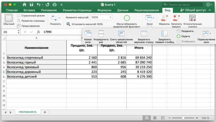
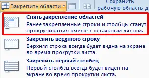
As an observant reader may have noticed, in the screenshot describing how to freeze one row, the third button from the left is labeled not as “Freeze regions”, but as “Unpin regions”. If you click it, you can unfreeze both a line and several lines. Here is such a universal button.
In simple words, the sequence of actions is as follows:
- Click on the “View” tab on the ribbon.
- Find the “Window” button there.
- “Click on the “Unpin areas” button.
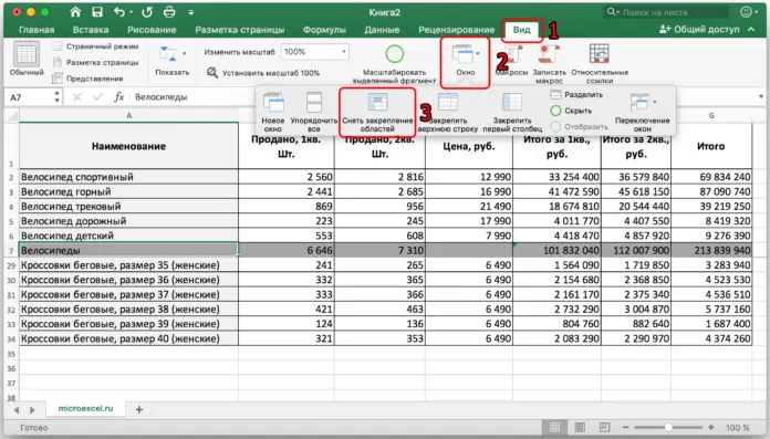

4
As you can see, just three clicks with the left mouse button are enough to do what you need. After that, the table will look as if it did not perform any operations to freeze the rows. And when scrolling, the line will simply move up until it leaves the computer monitor at all.
How to freeze a column in Excel
Suppose we needed to transpose the table and now the headings are placed in rows. Or we have any other document where information is placed not from top to bottom, but from left to right. In this case, you need to scroll horizontally and, therefore, it would be convenient to freeze the first column. Is it possible? Yes? Is it possible to pin several of them? And you’ll find out very soon.
How to freeze more than one column in a table?
It may turn out that you need to freeze several columns at once. To do this, you need to left-click on the very first cell of the column immediately following the last one you want to freeze. For example, if you need to fix two columns, then the cursor should be placed on cell C1, if there are three – D1 and then follow the same logic. We will try to freeze three cells, so we put the cursor on cell D1.
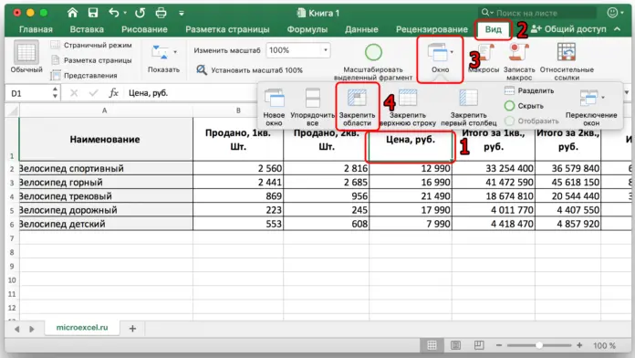
The sequence of actions is almost the same as in the examples described above. In the same way (we are now talking about new versions of Excel), you need to open the “View” tab, then the item “Freeze areas”, and then “Freeze areas”. The only difference compared to line pinning is the different cursor position.
In the above screenshot, for better understanding, numbers are drawn describing the sequence of actions.
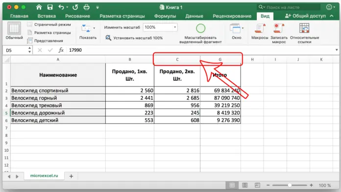
Now the first columns will always be shown, no matter how far horizontally the Excel spreadsheet is scrolled.
The sequence of actions in older versions is the same. The only exception is that instead of the “Window” button, you need to find a group of buttons with the same name on the “View” tab. There will be a “Lock Areas” button and an item of the same name in the pop-up menu.

How to freeze the first column?
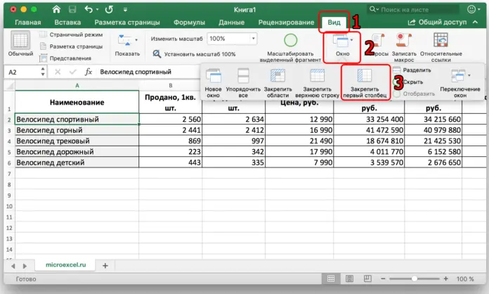
There is a corresponding Excel function to freeze the first column. It is located in the same place as the options for pinning rows or regions. Only in the latest versions is already closer to the right edge, being the fifth from the left. This is the Freeze First Column option.
To summarize briefly what needs to be done, then the following steps must be taken:
- Open the “View” tab (in all versions of Excel starting from 2007).
- Go to the Window group. This is done differently depending on the version of the program. If this is Excel 2007 or 2010, then just in the “View” tab there is a set with signatures. Among them there will be a set of buttons, signed as “Window”. You need to move the mouse cursor there. If a person works in new versions, then you need to click on the “Window” button, and a pop-up menu will open with the same options.
- There you need to find the button “Freeze the first column”.
Everything, after performing these actions, a person can scroll horizontally on the sheet, and the first column will still be displayed.
How to unfreeze a column(s)
Once all operations on the table have been completed, it may be necessary to unfreeze the columns. Then the table will look the same as before using this function. To do this, you must also go to the “View” tab, where you open the “Window” group of functions. We are again interested in the “Unpin regions” button. As you can see, it is universal, removing the pinning of both columns and columns (or both of them, if it was set like that).
How to freeze row and column at the same time
After we already know which buttons are where in different versions of Excel, let’s look at row and column pinning at the same time. Savvy readers might already have guessed how to do this, but let’s do a little check.
Imagine that we are faced with the task of fixing not just a row and a column, but two whole rows and columns
To do this, you need to find a cell that will be both the first right and the first bottom after the row and column, which you need to fix, respectively, and then click on it.
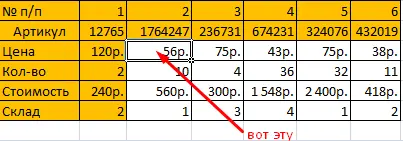
After that, you need to click on the “Freeze areas” button, which is located either in the drop-down menu with the same name or in the “Window” group, depending on the version of the spreadsheet program you are using.
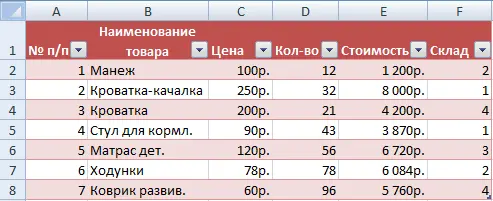
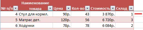
After that, a table appeared in front of us, which contains the articles of goods, and their numbers, and the price, and the quantity of the first, with which you can compare the rest.
How to remove pinned area
In all versions of Excel, after at least one of the regions has been frozen (even if it consists of only one row or column), the “Unfreeze regions” menu appears in the place where the “Freeze regions” button used to be.
After clicking this button, the sheet will look the same as before.
Important! In older versions of Excel (before 2003), you can find this function in the “Window” menu. At the same time, instead of the ribbon, there is a quick access panel, through which you can also remove the pinning in case of frequent use of this function.
As you can see, there is nothing difficult in fixing a row or column if necessary. All settings are intuitive, and a person with little experience can easily figure it out without instructions. But if you need to save time, then we hope this tutorial helped you understand what to do to anchor a row and column (or several rows and columns) to the edge of the document.
There are several other mechanisms that allow more professional processing of large amounts of data.