Contents
While working in Excel, along with adding and processing data, it is very important to present the information in the best possible way (color, size, font type, borders, fill, alignment, etc.), so that it is as informative and easy to perceive as possible. This will help formatting the table, with which, among other things, you can set the data type so that the program can correctly identify certain types of values in the cells. In this article, we will look at how formatting is performed in Excel.
Transformation into a “Smart Table”
By selecting a specific data area in the table, you can use such an option as auto-formatting. Excel will automatically convert the selected range to a table. Here’s how it’s done:
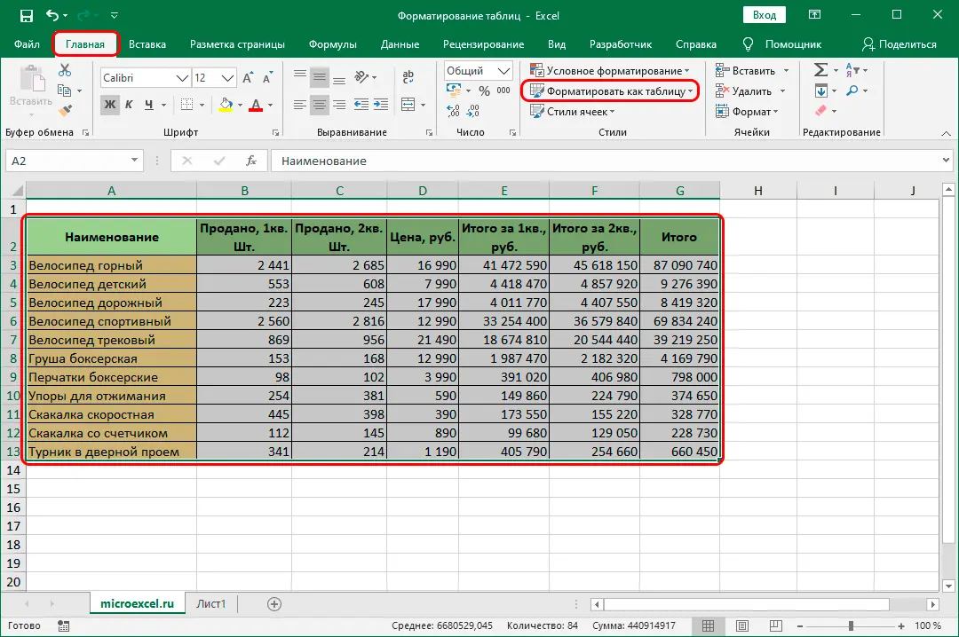
- We select the necessary elements. On the ribbon of the program we find a group of tools “Styles” (tab “Home“) and press the button “Format as table”.

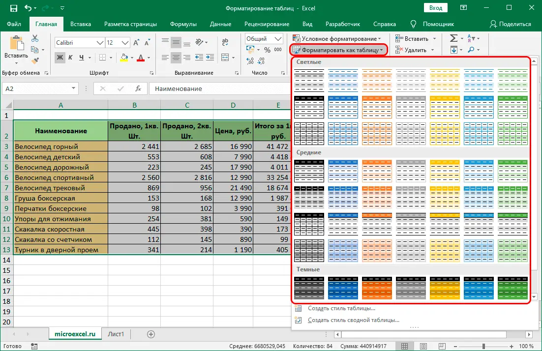
- A list of different styles with predefined settings will open. We can choose any of them by clicking on the option we like.

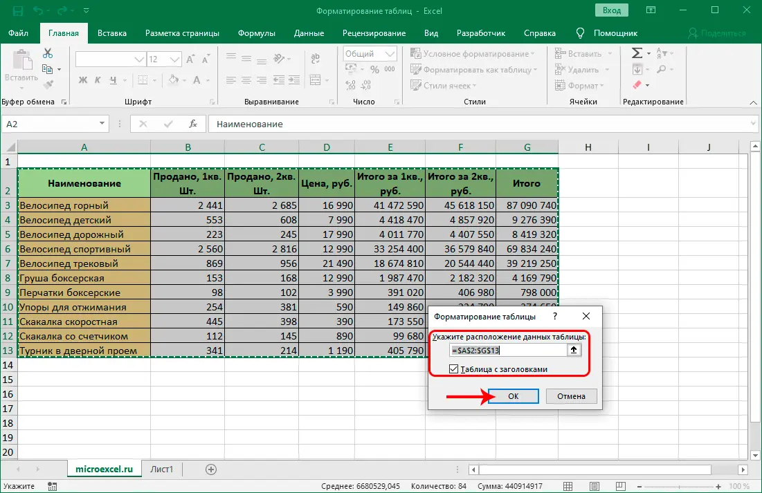
- An auxiliary window will appear on the screen, where the coordinates of the range selected in the first step will be displayed. If necessary, cell addresses can be corrected (manually or by re-selecting the required area in the table itself). If there is a table header in the selection, be sure to put it in front of the item “Table with headers” tick. Next click OK.

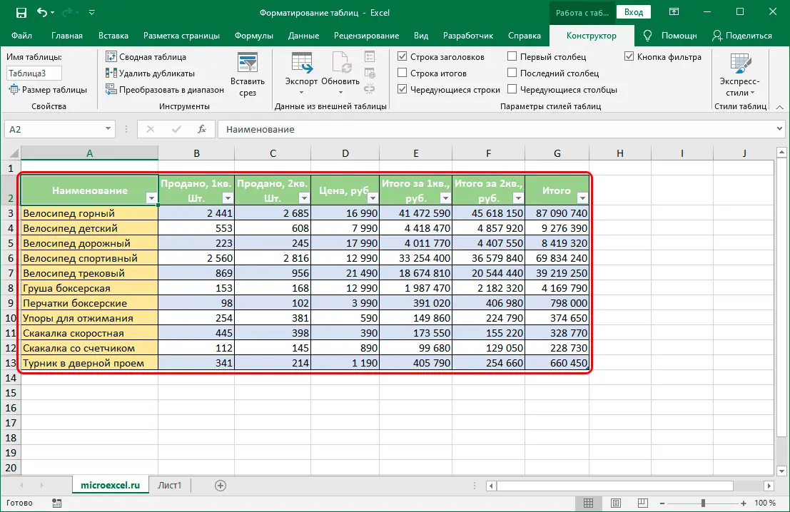
- As a result, our table is transformed into the so-called “smart table”.

Manual formatting
Despite such a useful option, discussed in the section above, some users prefer to independently determine the appearance of their table and give it exactly the settings that they consider the most optimal and appropriate. You can do this in different ways.
In the Format Cells window
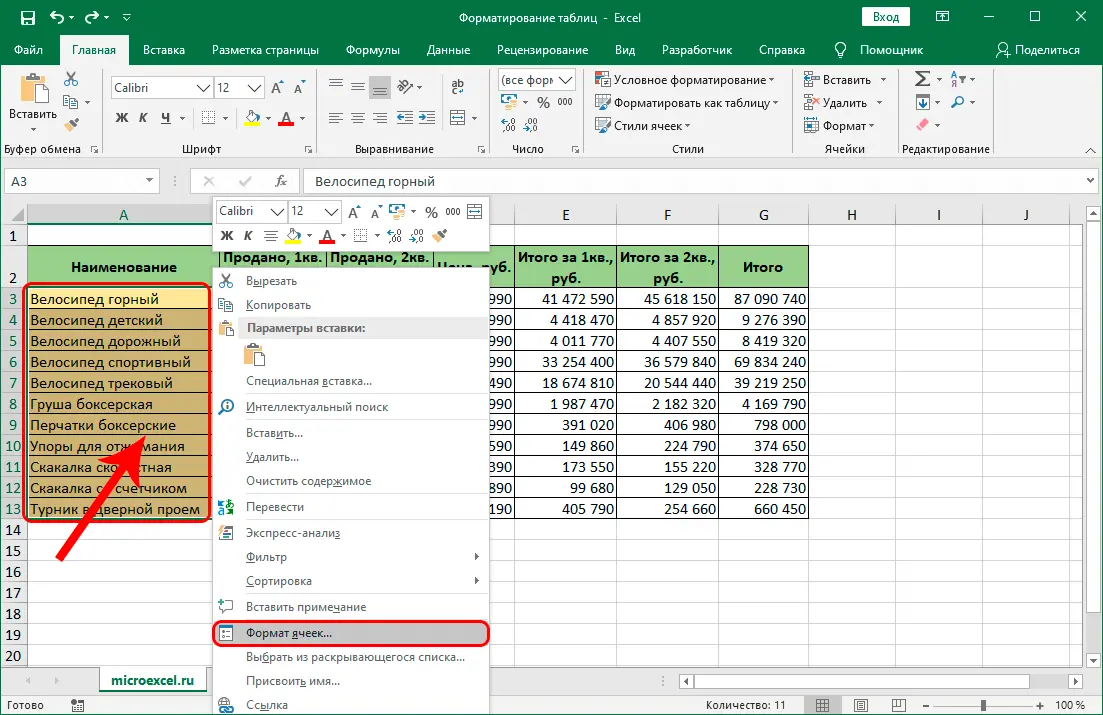
- We make a selection of the necessary elements to which we want to apply formatting, after which we right-click on the selected area. In the list that appears, click on the line “Cell Format”.

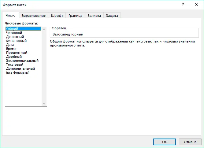
- A window will appear with formatting options for selected cells, in which we can set many settings in different tabs.

Using the Ribbon Tools
For formatting, you can use the tools that are located on the program ribbon, and the most popular ones are presented in the main tab. To apply a particular tool, just click on it, after selecting the required range of cells in the table.

Data type selection
Before you start working with data, you need to set the correct format for them, so that it is visually easier to perceive the information, and also so that the program correctly identifies and uses it when processing values and performing various calculations.
Cell Format window
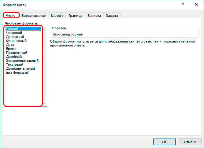
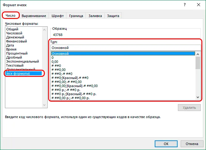
In the cell formatting window, you can make the required settings in the tab “Number”. In the list of available number formats, select one of the following options below:
- General;
- Numerical;
- Monetary;
- Financial;
- Date;
- Time;
- Percentage;
- Small;
- Exponential;
- Text;
- Additional;
- (all formats).

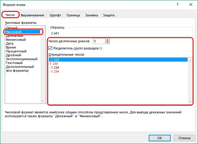
After we have made a choice, for almost all data types (except for general and text formats), the program will offer to set detailed parameters in the right part of the window.
For example, for a numeric format, you can:
- set the number of decimal places after the decimal point;
- determine if a thousands separator is needed;
- choose how negative numbers will be displayed.

This tool is convenient in that we can immediately see exactly how the data in the cell will be displayed – just look at the area “Sample”.
In “all formats” we can choose one of the data format subtypes or specify our own by using the field of the same name to enter a value, however, such a need arises extremely rarely.
Ribbon Tools
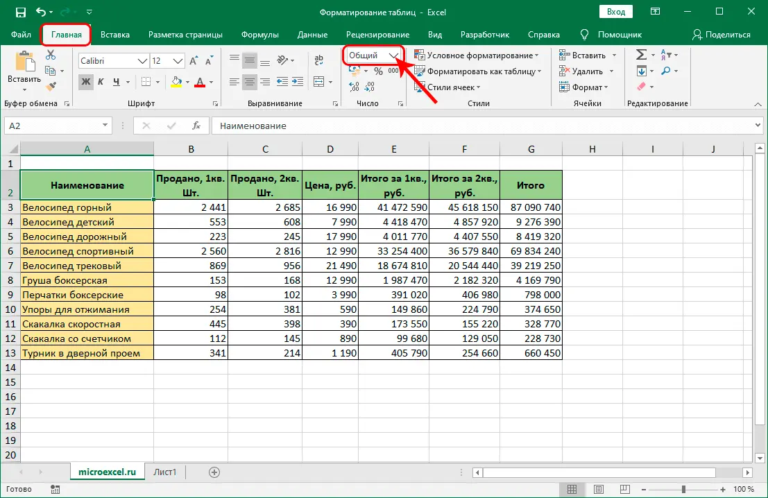
If you wish, you can set the data type using the tools on the program ribbon (tab “Home”).
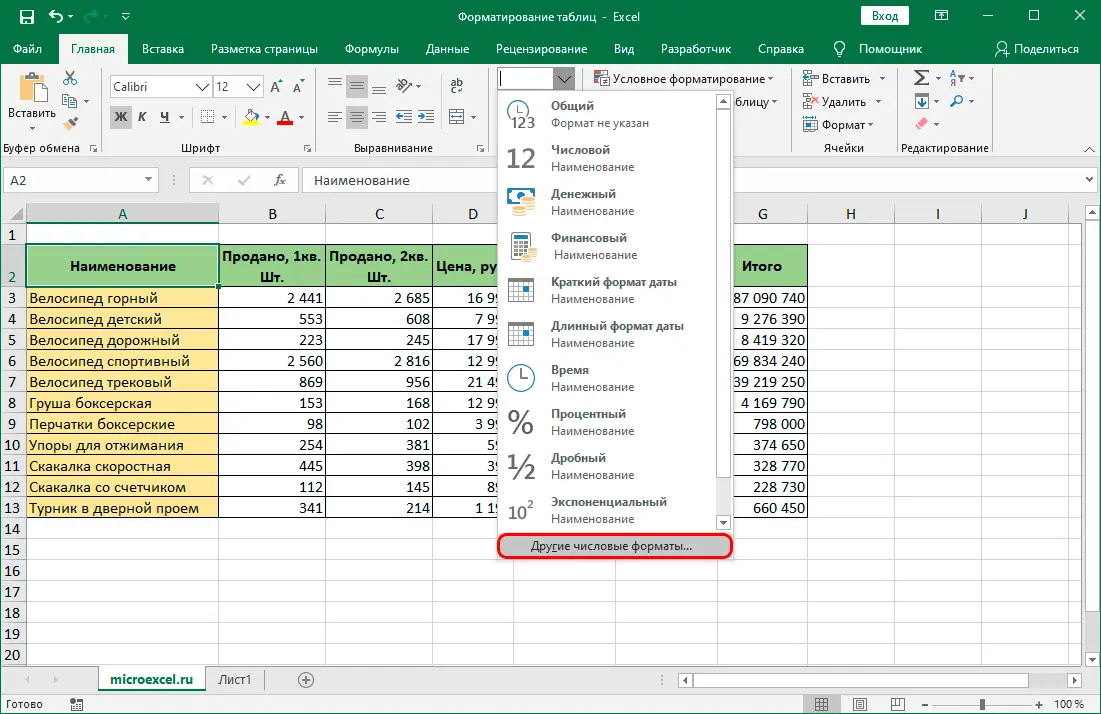
- Finding a group of tools “Number” and click on the down arrow next to the current value.

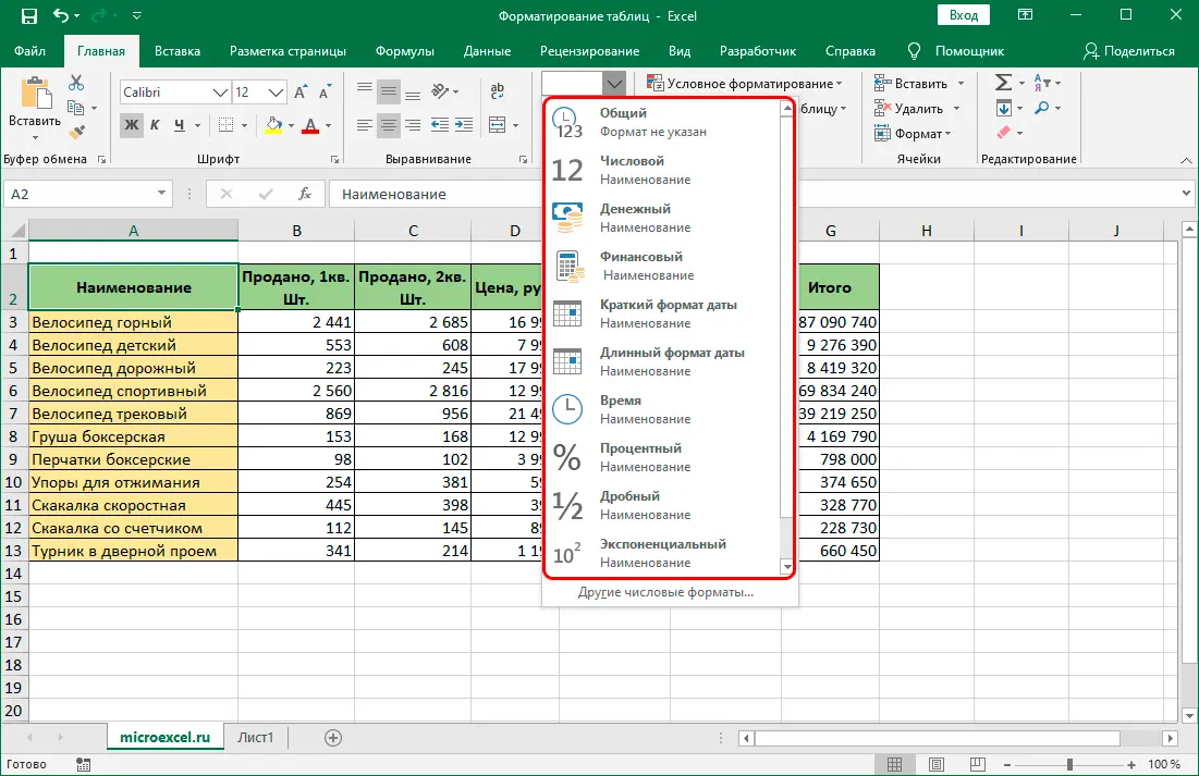
- Select one of the options from the drop-down list.

However, unlike the formatting window, in this case there is no possibility to set additional parameters. Therefore, if such a need arises, click on the option “Other number formats”, then a window will open “Cell Format”, which we have already discussed earlier.
Content alignment
You can also perform alignment both in the cell formatting window and in the main tab of the program using the tools on the ribbon.
Cell Format window
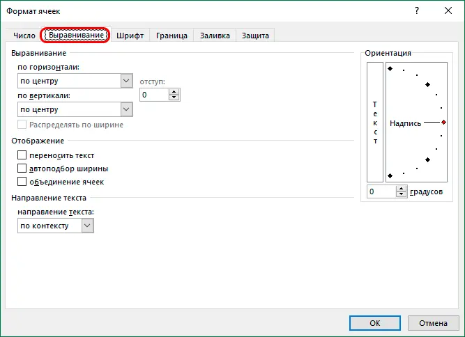
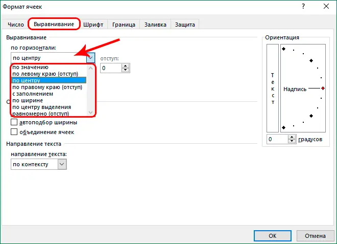
Switching to the tab “Alignment” we will get an extensive set of parameters, including:
- horizontal alignment;
- vertical alignment;
- indent;
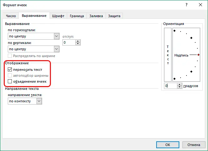
- display options:
- text wrapping;
- autowidth;
- cell merging;
- text direction;
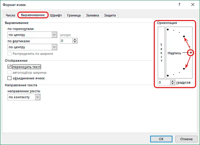
- orientation.

The settings of some parameters are performed by selecting the appropriate value from the proposed list, which is opened by clicking on the current option (for example, for horizontal alignment).
For others, simply ticking the box is enough.
Let’s dwell on the orientation of the text separately. We can choose the position of the text (horizontally or vertically) and adjust its angle by shifting the corresponding point of the line with the left mouse button pressed or by entering the desired degree in the field specially provided for this.
Ribbon Tools
There is a special group of tools on the program ribbon “Alignment”where you can make the most popular settings.
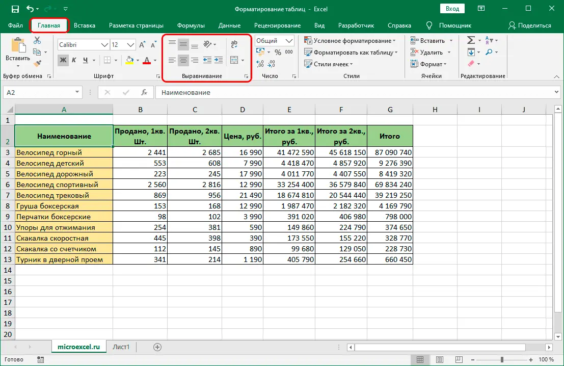
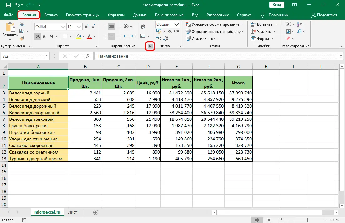
If they are not enough to get into the tab “Alignment” cell formatting window, you can click on the icon (in the form of an unfinished square with an arrow inside) which is located in the lower right part of the toolbox.
Font setting
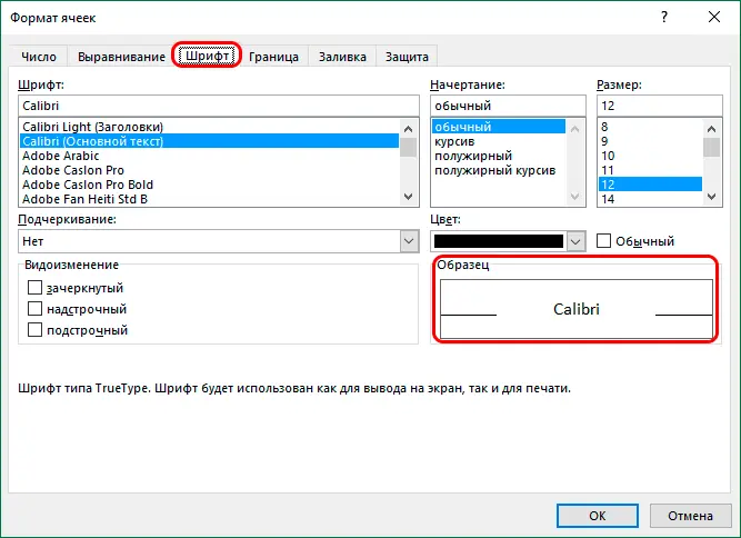
Going to the tab “Font” in the format window we will access the relevant options. Here you can set:
- font type;
- style (regular, italic, bold, or bold italic);
- the size;
- Colour;
- underscore (single or double);
- modification (strikethrough, superscript or subscript).

You can track the result taking into account the settings made here, in a special block reserved for this “Sample”.
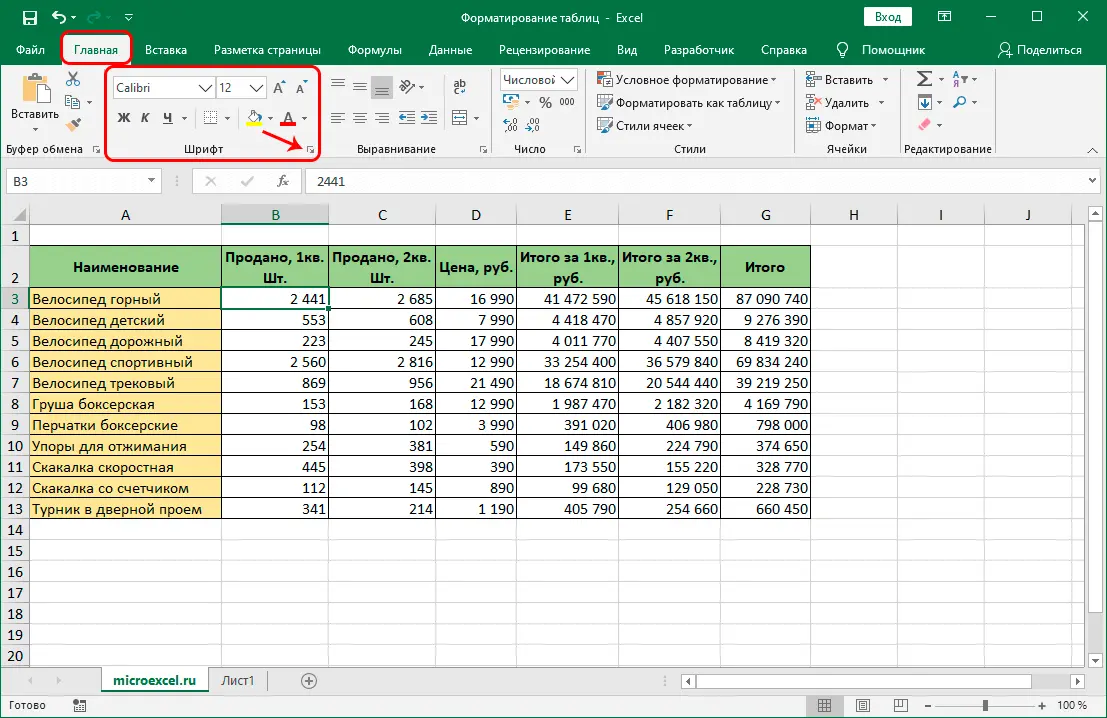
On the tool tape there is also a separate group of tools for setting the font. To go to more detailed parameters in the cell formatting window, you need to click on a special icon in the lower right part of this block.
Borders and lines
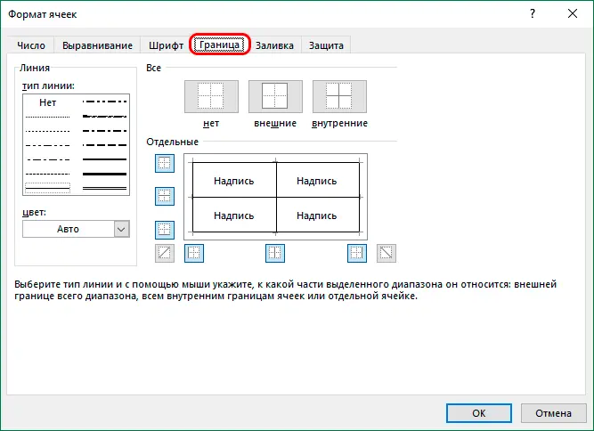
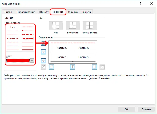
In the “Cell Format” you can also make border settings by going to the tab of the same name, which contains the following options:
- line type;
- Colour;
- display option:
- no;
- external;
- internal (if two or more cells are selected).

It is also possible to fine-tune the borders in the block “Separate”, selecting the thickness, type and color for each line. First, set the desired parameters, then click on the border to which we want to apply them.
On the program feed there is no special group of tools for setting borders. In the block “Font” there is only one button that opens the list of available options.
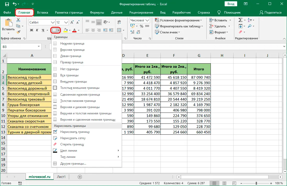
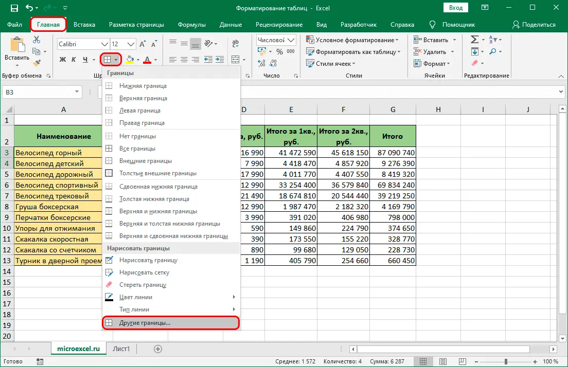
Selecting an item “Other Frontiers” we’ll get into the tab “Borders” the formatting window described above.
Filling cells
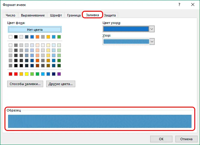
If we go to tab “Filling” in the window “Cell Format”, we will have access to the following settings:
- background color of selected cells;
- selecting a pattern as a fill;
- pattern color.

You can track the result in a special field “Sample”.
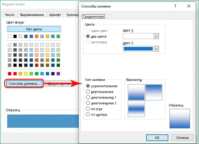
By clicking on the button “Fill Methods” you can get into the gradient fill settings (although this option is not often used).
On the toolbars programs, as in the case of borders, only one button in the group is provided for filling “Font” (tab “Home”), clicking on which will open a list of possible options.
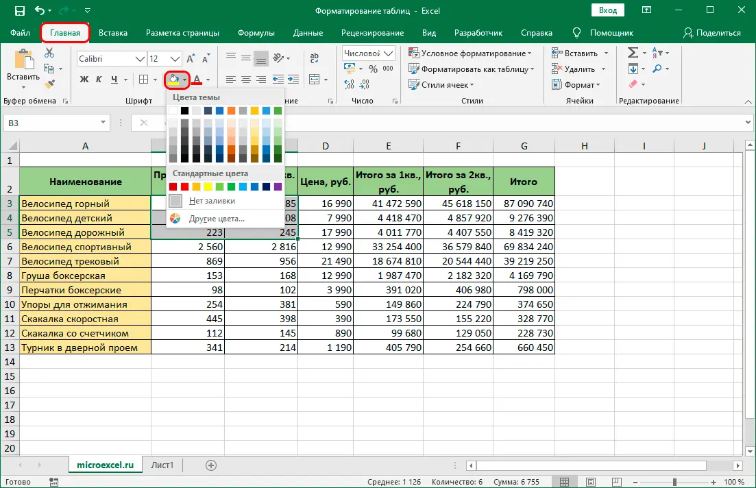
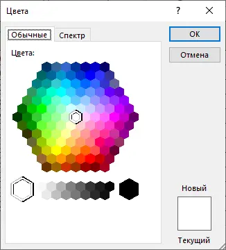
When choosing an item “Other colors” a window will open in which we can adjust the color in more detail in one of two tabs – “Color” or “Spectrum”.
Data protection
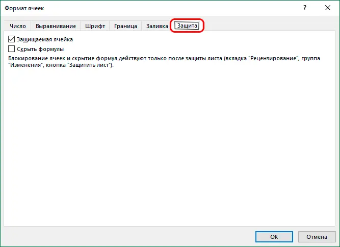
With this function, you can protect the contents of the cells, so it is also available in the formatting window in a separate tab.
Here we can by checking the box:
- hide formulas;
- protect cells.

These options only work after the sheet has been protected. You can learn more about how to protect data in Excel in our article -.
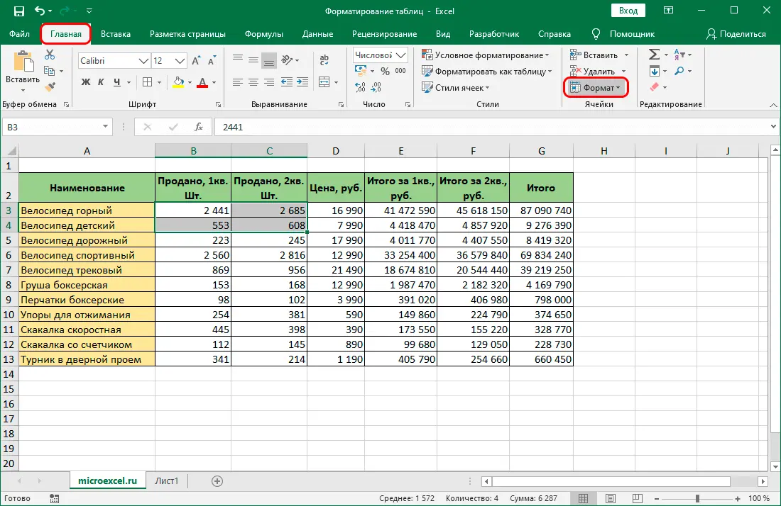
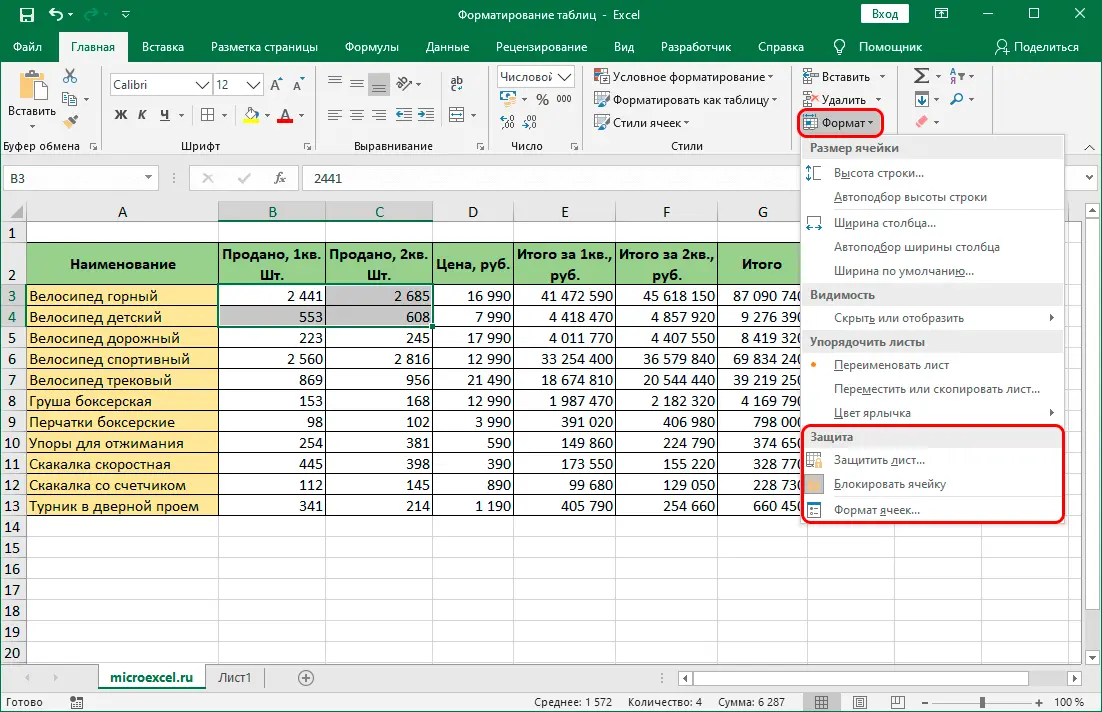
On the toolbar, you can find these options in the group “Cells” (tab “Home”) by pressing the button “Format”.
In the list that opens, there is a block called “Protection”. There is also an option to immediately enable sheet protection. If you need to go to the window “Cell Format”, you should click on the button of the same name.
Conclusion
In Excel, the user is offered an extensive list of tools for customizing the appearance of the table, as well as determining the type of data, which is extremely important for the program to correctly recognize them. Most popular settings are placed on the program ribbon in the “Home” tab. For more detailed settings, you need to use the cell formatting window, which is launched through the context menu of selected elements.


