How to flip an excel spreadsheet

Table transposition is a feature that not all Microsoft Excel users know about. It is intended for cases where you need to change the orientation of a range of cells from vertical to horizontal or vice versa. The program also allows you to rotate one column so that the data goes in reverse order – this is useful if the information is entered incorrectly. Let’s figure out how to change the location of the data on the sheet without having to rewrite the whole thing.

Transpose an Excel spreadsheet with Paste Special

There are situations when all the data is already entered in the table, but it was necessary to arrange the contents of the header vertically. To do this, you can use the Paste Special tool – its menu contains several settings that allow you to adjust the insertion of a table in a new place. Let’s take any table where there is a header and try a special insert on it.

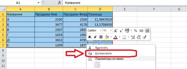
1. Select the entire range of cells and copy it using the key combination “Ctrl + C”. You can also right-click and select Copy from the context menu.

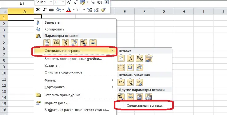
2. On a new sheet or in another part of the same sheet, we find an empty space where you want to insert a table. Press the right mouse button, placing the cursor on one of the cells, and select the “Paste Special” item. In some versions of Microsoft Excel, hovering over this menu item immediately opens options, but you need to find the “Paste Special” item at the bottom of the additional menu and click on it.

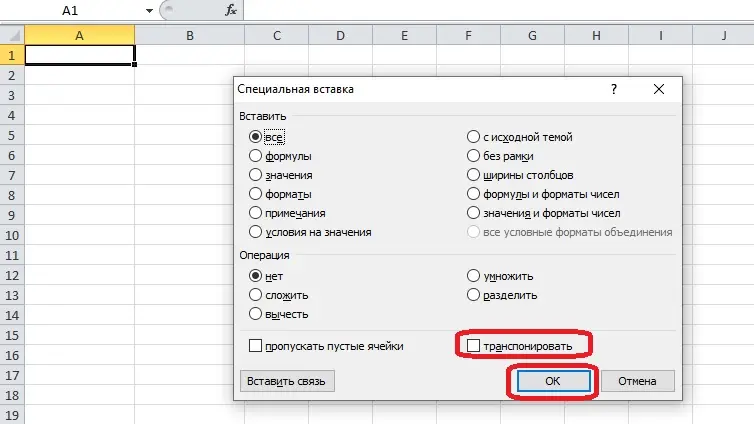
3. The dialog box contains several options that allow you to insert individual data from the table in a new location. Put a checkmark in the “Transpose” box and click “OK”.

4. Now the table header is in the first column, and the data has moved from there to the top row. On such a table, the difference between sales volumes is also clearly visible.

How to flip a table with a function

The Function Wizard contains a formula that can be used to swap rows and columns in a table. You will have to copy the data again and paste it into another range of cells to see the changes.

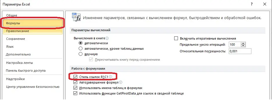
1. Go to “Options” and in the “Working with formulas / Formulas” section, check the box “Reference style R1C1”. This will be needed in the future for correct work with the formula. If this step is not passed, it will not be possible to add an array of data to the function.

2. We determine the place where the modified table will be located and add the TRANSPOSE function to the first cell. The formula can be found in the Function Wizard or written by hand – all you need is a letter and parentheses.

Pay attention! If you use the Function Wizard menu to search for formulas, you should open the “References and arrays” category. When writing a formula by hand, be sure to put an equal sign at the beginning.

3. Go to the sheet with the initial table and select it so that the range of cells gets into the formula. Then click “OK”. The table hasn’t migrated completely yet, but that’s ok – two more steps are required.

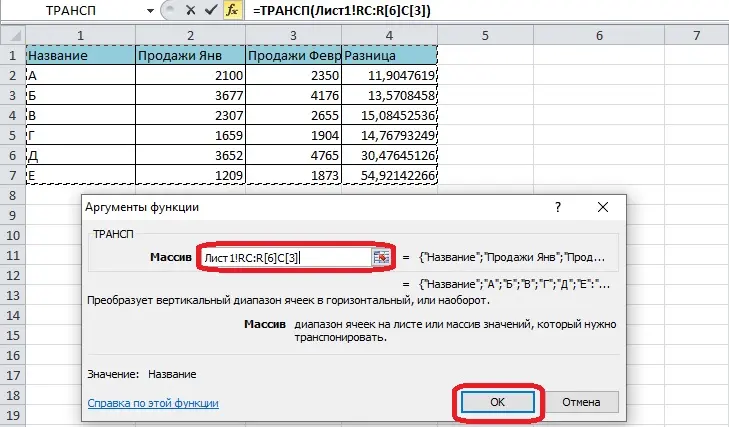
4. On the sheet with the function, select the cells in the ratio in which they will be after the flip. For example, in the example table, there are 7 rows and 4 columns, which means that you need to select 4 rows and 7 columns.

5. Let’s use the keyboard shortcut to make the formula work. First, press F2 – if functions are set to this button, find the key that stops them from working and hold it down. The formula in the cell expands. Next, quickly press three keys: Ctrl, Shift, Enter. An inverted table will appear in the selected range.

Transpose using PivotTable

Pivot tables help in many ways when using Excel. This option also comes in handy when transposing. With a PivotTable, you can only move columns in place of rows, not vice versa. This method also has advantages – users can filter the data in the table.

1. Highlight the source range of cells with the cursor.
2. Go to the “Insert” tab on the toolbar and find the “Pivot Table” button.

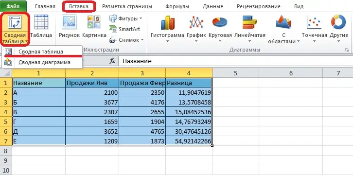
3. Customize the formation of the pivot table in the dialog box. It indicates the range of cells – it is already selected – and the insertion point. Select a new sheet to easily manage your new range of data.
4. We distribute the fields in the list by categories. The contents of the columns must refer to rows, and vice versa.

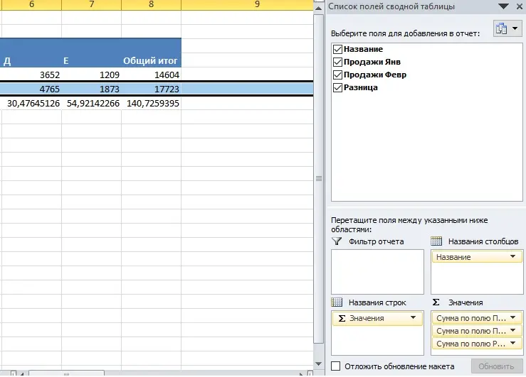
5. Open the Design tab and turn off grand and subtotals for rows and columns.

6. The result is a table with the same values, but the rows and columns have changed their position.

How to flip one column with a function

If your Excel spreadsheet has a column with values ​​in reverse order, you can flip it using the Function Wizard. There are two formulas to help you flip a column upside down.

1. We insert in the cell with which the inverted column begins, the function OFFSET or INDEX. Feel free to use these templates, but don’t forget to insert values ​​that match the location of the cells in your table: =OFFSET($A$8,(ROW($A$2)-ROW());) or =INDEX($A$2:$A$8;ROWS(A2:$A$8)).
2. For example, let’s use the OFFSET function – add it to a cell and press Enter.

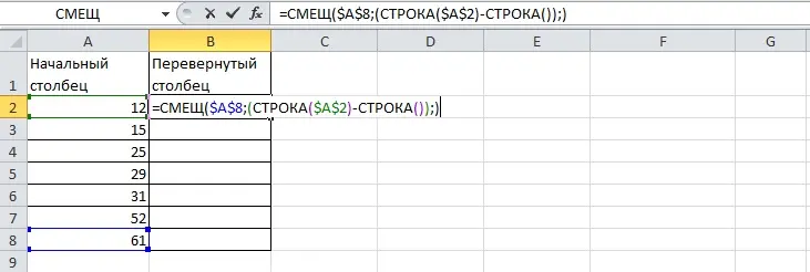
3. We hold the fill handle – the black square in the lower right corner of the cell – and drag the selection to the end of the column. All cells will be filled in according to the plan, that is, in reverse order.

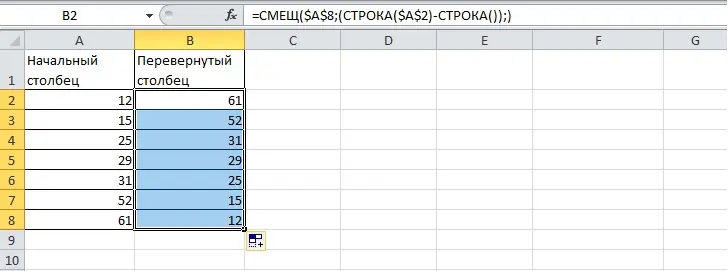
4. The result of filling a column using the INDEX function looks like this:

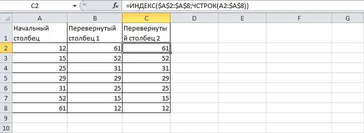
Important! It is not necessary that the columns are adjacent, the links in the formulas still lead to the desired cells. This knowledge will come in handy to make an inverted column outside of a whole table.

Conclusion

Most table flipping, or transposing, methods work both ways. The user can make a vertically oriented range of cells horizontal, or make the header of the row names. Only pivot tables are not suitable for two-way transposition. The easiest way to rotate a table is to use Paste Special.