


Contents
Many novice Excel users often have a question: what is an Excel formula and how to enter it into a cell. Many even think why it is needed. To them, Excel is a spreadsheet. But in fact, this is a large multifunctional calculator and, to some extent, a programming environment.
Concept of formula and function
And all the work in Excel is based on formulas, of which there are a huge number. At the heart of any formula is a function. It is a basic computational tool that returns a value depending on the transmitted data after it has been pre-processed.
A formula is a set of logical operators, arithmetic operations and functions. It does not always contain all of these elements. The calculation may include, for example, only mathematical operations.
In everyday speech, Excel users often confuse these concepts. In fact, the line between them is rather arbitrary, and both terms are often used. However, for a better understanding of working with Excel, it is necessary to know the correct values.
In fact, the terminological apparatus is much broader and includes many other concepts that need to be considered in more detail.
- Constant. This is a value that remains the same and cannot be changed. This could be, for example, the number Pi.
- Operators. This is a module required to perform certain operations. Excel provides three types of operators:
- Arithmetic. Needed to add, subtract, divide and multiply multiple numbers.
- Comparison operator. Needed to check if the data meets a certain condition. It can return one value: either true or false.
- Text operator. It is only one, and is needed to concatenate data – &.
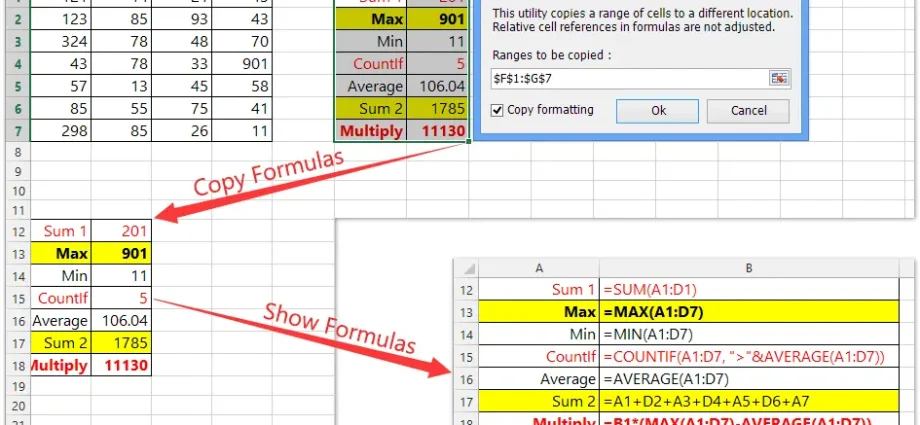
- Link. This is the address of the cell from which the data will be taken, inside the formula. There are two types of links: absolute and relative. The first do not change if the formula is moved to another place. Relative ones, respectively, change the cell to the adjacent or corresponding one. For example, if you specify a link to cell B2 in some cell, and then copy this formula to the adjacent one on the right, the address will automatically change to C2. The link can be internal or external. In the first case, Excel accesses a cell located in the same workbook. In the second – in the other. That is, Excel can use data located in another document in formulas.
How to enter data into a cell
One of the easiest ways to insert a formula containing a function is to use the Function Wizard. To call it, you need to click on the fx icon a little to the left of the formula bar (it is located above the table, and the contents of the cell are duplicated in it if there is no formula in it or the formula is shown if it is. Such a dialog box will appear.
There you can select the function category and directly the one from the list that you want to use in a particular cell. There you can see not only the list, but also what each of the functions does.
The second way to enter formulas is to use the corresponding tab on the Excel ribbon.
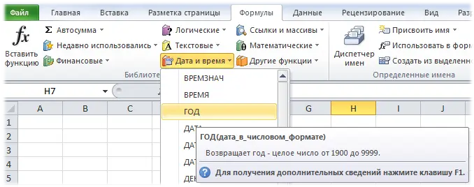
Here the interface is different, but the mechanics are the same. All functions are divided into categories, and the user can choose the one that suits him best. To see what each of the functions does, you need to hover over it with the mouse cursor and wait 2 seconds.
You can also enter a function directly into a cell. To do this, you need to start writing the formula input symbol (= =) in it and enter the name of the function manually. This method is suitable for more experienced users who know it by heart. Allows you to save a lot of time.
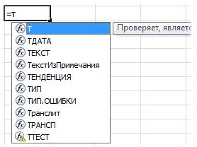
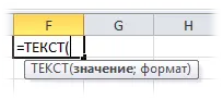
After entering the first letters, a list will be displayed, in which you can also select the desired function and insert it. If it is not possible to use the mouse, then you can navigate through this list using the TAB key. If it is, then simply double-clicking on the corresponding formula is enough. Once the function is selected, a prompt will appear allowing you to enter the data in the correct sequence. This data is called the function’s arguments.
If you are still using Excel 2003 version, then it does not provide a drop-down list, so you need to remember the exact name of the function and enter data from memory. The same goes for all function arguments. Fortunately, for an experienced user, this is not a problem.
It is important to always start a formula with an equal sign, otherwise Excel will think that the cell contains text.
In this case, the data that begins with a plus or minus sign will also be considered a formula. If after that there is text in the cell, then Excel will give an error #NAME?. If figures or numbers are given, then Excel will try to perform the appropriate mathematical operations (addition, subtraction, multiplication, division). In any case, it is recommended to start entering the formula with the = sign, as it is customary.
Similarly, you can start writing a function with the @ sign, which will be automatically changed. This input method is considered obsolete and is necessary so that older versions of documents do not lose some functionality.
The concept of function arguments
Almost all functions contain arguments, which can be a cell reference, text, number, and even another function. So, if you use the function ENECHET, you will need to specify the numbers that will be checked. A boolean value will be returned. If it is an odd number, TRUE will be returned. Accordingly, if even, then “FALSE”. Arguments, as you can see from the screenshots above, are entered in brackets, and are separated by a semicolon. In this case, if the English version of the program is used, then the usual comma serves as a separator.
The input argument is called a parameter. Some functions do not contain them at all. For example, to get the current time and date in a cell, you need to write the formula =TATA (). As you can see, if the function does not require the input of arguments, the brackets still need to be specified.
Some features of formulas and functions
If the data in the cell referenced by the formula is edited, it will automatically recalculate the data accordingly. Suppose we have cell A1, which is written to a simple formula containing a regular cell reference = D1. If you change the information in it, then the same value will be displayed in cell A1. Similarly, for more complex formulas that take data from specific cells.
It is important to understand that standard Excel methods cannot make a cell return its value to another cell. At the same time, this task can be achieved by using macros – subroutines that perform certain actions in an Excel document. But this is a completely different topic, which is clearly not for beginners, since it requires programming skills.
The concept of an array formula
This is one of the variants of the formula, which is entered in a slightly different way. But many do not know what it is. So let’s first understand the meaning of this term. It is much easier to understand this with an example.
Suppose we have a formula SUM, which returns the sum of the values in a certain range.
Let’s create such a simple range by writing numbers from one to five in cells A1:A5. Then we specify the function =SUM(A1:A5) in cell B1. As a result, the number 15 will appear there.
Is this already an array formula? No, although it works with a dataset and could be called one. Let’s make some changes. Suppose we need to add one to each argument. To do this, you need to make a function like this:
=SUM(A1:A5+1). It turns out that we want to add one to the range of values before calculating their sum. But even in this form, Excel will not want to do this. He needs to show this by using the formula Ctrl + Shift + Enter. The array formula differs in appearance and looks like this:
{=SUM(A1:A5+1)}
After that, in our case, the result 20 will be entered.
There is no point in entering curly braces manually. It won’t do anything. On the contrary, Excel will not even think that this is a function and just text instead of a formula.
Inside this function, meanwhile, the following actions were carried out. First, the program decomposes this range into components. In our case, it is 1,2,3,4,5. Next, Excel automatically increments each of them by one. Then the resulting numbers are added up.
There is another case where an array formula can do something that the standard formula cannot. For example, we have a data set listed in the range A1:A10. In the standard case, zero will be returned. But suppose we have such a situation that zero cannot be taken into account.
Let’s enter a formula that checks the range to see if it is not equal to this value.
=МИН(ЕСЛИ(A1:A100;A1:A10))
Here there is a false feeling that the desired result will be achieved. But this is not the case, because here you need to use an array formula. In the above formula, only the first element will be checked, which, of course, does not suit us.
But if you turn it into an array formula, the alignment can quickly change. Now the smallest value will be 1.
An array formula also has the advantage that it can return multiple values. For example, you can transpose a table.
Thus, there are a lot of different types of formulas. Some of them require simpler input, others more complex. Array formulas can be especially difficult for beginners to understand, but they are very useful.