How to draw a pie chart in Excel

If you’re just getting started with Excel and need to visualize information or present it visually in a presentation, you’ve come to the right place. In this pie chart tutorial, we’ll show you how to draw, cut, and rotate charts, add and edit labels, show percentages, and many other Excel tricks.

A pie or pie chart is a convenient way to show the percentage of individual components that together make up a whole. The full circle of the sector graph represents 100% of the whole, and its sectors are the constituent parts of the whole.

Users simply love to insert graphs and charts into presentations, however, data visualization experts are of the opposite opinion. The fact is that human vision is unable to correctly evaluate angles, which makes pie charts much less visual.

However, humanity has not yet come up with a worthy replacement for diagrams, so the only way out is to learn how to compose them correctly. Drawing a pie chart from scratch while maintaining all the angles and percentages is quite difficult. But, fortunately, Excel allows you to do this in a matter of minutes, and the result is an attractive and professional looking result.

How to draw a chart in Excel

Forming a chart in Excel is an extremely simple process that requires only a couple of mouse clicks. The user will only need to successfully distribute information in Excel cells and choose the most optimal type of graph for displaying it.

1. Data formatting for the chart

To form a sector graph, you must first collect data in cells located in one row, that is, located in a common column or line. The fact is that Excel allows you to translate only 1 series of data into a graph.

In addition to the column with the initial information, a column or line with the names of data categories is also used to draw up a graph. This is necessary in order for data category labels to appear directly on the chart.

In general, pie charts look more presentable when:

• To create them, only 1 row of cells with information was used.
• All numeric values ​​> 0.
• There are no blank columns or rows without information.
• The graph is divided into no more than 8 data categories. If there are too many parts, the diagram will be difficult to understand.

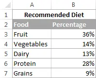
In this tutorial, we will create a pie chart based on the following input:

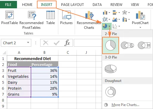
2. Insert a pie chart into a worksheet

After collecting the necessary information and inserting it into the worksheet, select it and go to the “Insert” tab. There will be several chart options. Choose the one that best suits your goals (more on the types of pie charts below).

For this example, let’s focus on a simple XNUMXD variant.

Council: In addition to columns or rows with numbers and category names, also capture their headings (eg, like “Recommended diet” in the screenshot above). In this case, the column and row headings will become the graph headings.

3. Pick a Chart Style (Optional)

Once you’ve drawn a pie chart, select the Design toolbar item, where there are several different chart styles to choose from. Pick a style that goes well with your input.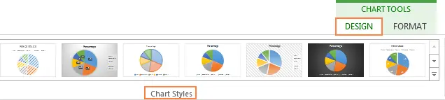

A standard flat chart looks like this: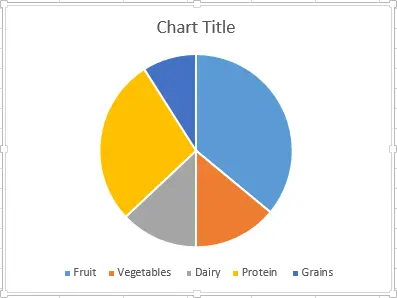

Agree, it looks pretty boring. It will not interfere with the headline, captions and a harmonious color palette. We will talk about this a little later, but for now, we will focus on the available types of pie charts.

Types of pie charts and their uses

In total, the program offers several types of sector charts:

• two-dimensional;
• three-dimensional;
• auxiliary circular or linear.

XNUMXD pie charts

This is the typical and most commonly used chart. The necessary tool for its formation is located in the “Insert” tab.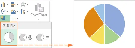

XNUMXD pie charts

Volumetric graphs are almost identical to flat ones. The only difference is that the XNUMXD chart has a Z axis and is visually displayed not from above, but from the side.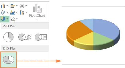

Having drawn a volumetric pie chart, you can freely rotate it along the coordinate axes, as well as set the perspective.

Auxiliary charts

If your graph consists of a lot of narrow fragments, for the sake of viewing convenience, it makes sense to create an auxiliary graph and display the least significant parts of the chart on it.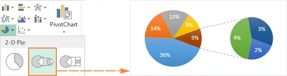

The auxiliary line chart performs the same function as the sector chart, however, it displays the selected sectors not in a circle, but in a column.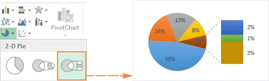

Auxiliary charts are created from the last three fragments of the original chart. And since this is not always optimal, the solution to the problem is the following: 

• Arrange the data from largest to smallest so that the cells with the smallest values ​​are always at the bottom of the list and thus appear in the auxiliary graph.
• Manually select the sectors to display in the auxiliary chart.

Selection of fragments for the auxiliary chart

To select sectors to transfer to the auxiliary chart, do the following:

1. RMB click on an arbitrary sector, and then LMB – on the “Data series format” item.
2. In the sidebar that appears, find “Row Options” and the drop-down menu for “Split Row”. The division takes place according to the following criteria:

• Position – moves the fragments that are located last to the auxiliary chart.
• Value – sets a numerical threshold for fragments. All fragments of the main chart that do not reach the specified threshold will be transferred to the secondary chart.
• Percent – largely identical to Value, but allows you to set only the minimum percentage of the sector relative to the entire chart.
• Other – allows you to manually select any sector of the chart and indicate whether they belong to the main or auxiliary chart.

In the vast majority of cases, the percentage threshold is the best sorting option. But it depends on the initial information of the graph, as well as on the personal preferences of the user. In the image below, the fragments are sorted by percentage: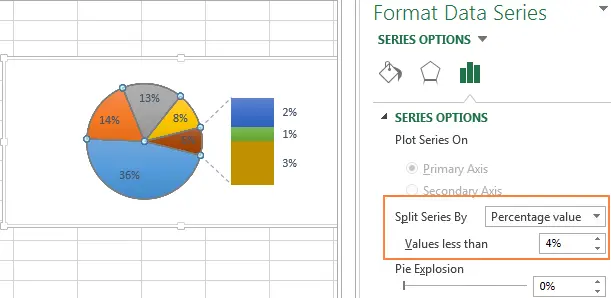

In addition, when creating an auxiliary chart, the following parameters must be configured:

• Distance between graphs. The percentage under this parameter displays the width of the subplot. To increase the gap, drag the setting slider to the right.
• Auxiliary chart size. This parameter is responsible for the diameter of the secondary chart. Drag the slider left or right to resize the graph, or enter the exact percentage directly.

Donut charts

When working with multiple data series that together make up a whole, a donut chart will be able to display them better than a pie chart. The problem is that in donut charts it is more difficult to estimate the proportions between fragments from different series, so if you need to draw the chart as clearly as possible, you should turn to other types of charts, such as a bar chart or line chart.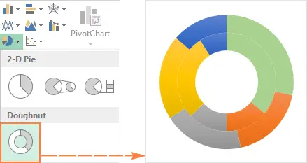

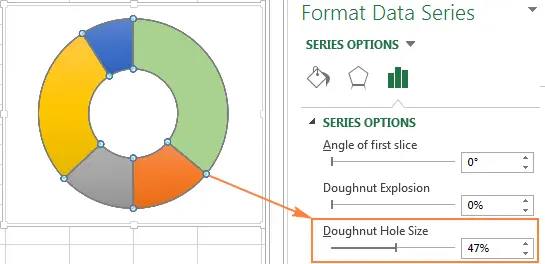
Donut inner diameter

When forming a pie chart, Excel makes it possible to adjust the size of its inner hole. You can do this in the following way:

1. Right-click on any part of the graph and select “Format Data Point”.
2. In the side menu that appears, find the “Row Options” section and change the diameter of the inner hole using the appropriate slider, or by entering the desired percentage value yourself.

Personalization of pie charts

If you only need a chart to quickly assess certain trends in your data, a simple flat chart will do just fine. However, if the visualization is needed for a presentation, it will not be superfluous to refine it a bit by adding a few details to it.

How to sign individual sectors

Let’s try to add labels to all sectors of the chart. To do this, click on the “+” sign to the right of the graph, and then click on the arrow next to “Data Labels”. Compared to other charts, pie charts have the largest number of labeling options available: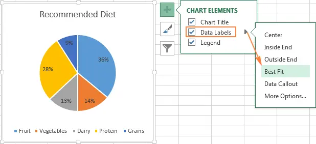

If you want to display labels outside the sectors, select the appropriate item in the “Data callout” list.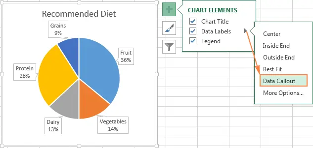

Council: If you add captions inside chart fragments, the standard black text will be difficult to read on dark fragments (see one of the screenshots above). For better readability, change the color of the text in such sectors to lighter (go to “Format” and find there “Text fill”). The hues of the chart sectors themselves are also customizable.

Displaying categories on chart fragments

If the sector chart consists of 3 fragments or more, then it makes sense to label the categories directly on them so that in the future people do not have to constantly check the legend. 

The easiest way to label categories on sectors is to select a ready-made layout in the tab “Constructor”, menu item “Express layout”. The first 4 layouts in the list include category labels, so you don’t have to add them manually: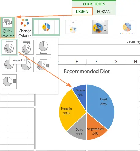

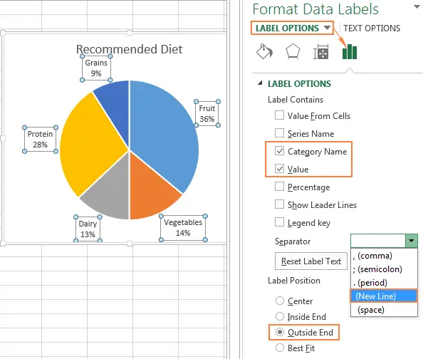
For additional design options, click the “+” to the right of the chart, and then click on the arrow opposite “Data Signatures” and then “Extra. options”. This will open a side menu on the right side of the screen. Go to “Signature Options” and check the box next to “Category Name”.

You may also find the following tricks useful:

• The list “Include in Signature” select the data you want to display in the labels (for example, the category name or value).
• In the graph “Separator” mark the way you want to separate the data (e.g. newline or semicolon).
• В “Label position” select the desired location of the labels (outside or inside the chart).

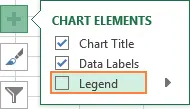
Council. When you add category labels to sectors, the legend is no longer needed. It can be disabled by clicking the “+” to the right of the graph and unchecking the box. “Legend”.

Displaying percentages on a pie chart

If the data on which the graph is based is specified in percentage values, then the % icon will be displayed automatically if you turn on “Data Signatures” в “Graphic Elements”, or check the box next to the item “Meaning” in the already well-known submenu “Data signature format”.

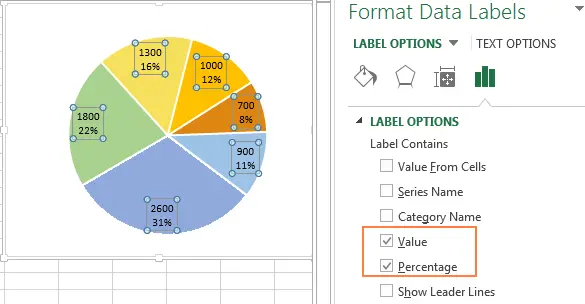
If the initial data is presented as numbers, then you can sign the sectors with both numerical and percentage values ​​(or both at the same time):

• Right-click on an arbitrary sector and select an item “Data Signature Format”.
• In the side menu, check the boxes “Meaning” or “Shares”, or both points at the same time, as in the screenshot below. The program will calculate the shares on its own with a total percentage equal to 100%.

Splitting the chart and extracting individual sectors

To visually highlight the sectors of an Excel chart, you can “cut” it, that is, remove the sectors at the same distance from the center of the chart. Or you can select individual sectors, “cutting off” them from the bulk of the diagram.

You can cut both flat and three-dimensional pie and donut charts:

Slicing a pie chart

The easiest way to cut the entire chart is to select all sectors with one click, and then move them away from the center without releasing the left mouse button.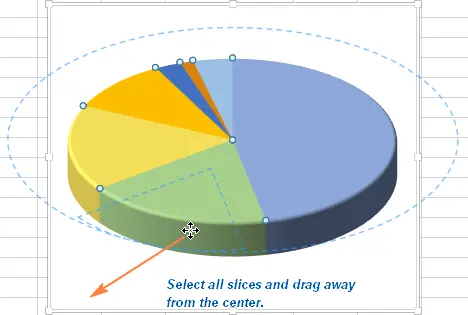

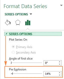
To slice the graph accurately, follow these steps:

1. Right-click on an arbitrary sector and select an item “Data Series Format”.
2. In the sidebar that opens, find “Row Options” and use the slider “Sliced ​​Pie Chart” to increase or decrease the gap between sectors. Alternatively, enter the desired percentage manually.

How to cut off a single sector from the chart

To focus on one specific sector, cut it off from the main body of the chart. As in the previous case, this is easy to do by dragging the sector with the mouse. Just click LMB on the fragment, and then click on it again to select only it, and drag it with the mouse away from the center.

You can also select the desired fragment, then right-click on it and select the item “Data Series Format”, where you can change the value of the parameter “Spot Cut”: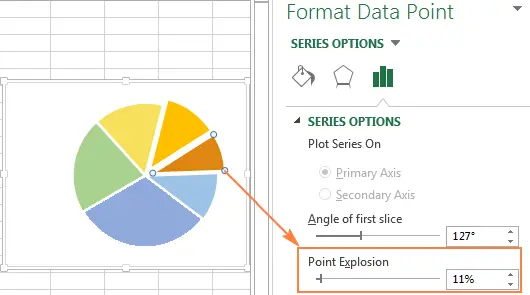

Note: If you need to select several fragments, then the process described above will have to be repeated for each individual sector. Excel does not allow you to select and cut several individual sectors at the same time. You can either cut the entire chart at once, or cut one sector at a time.

Pie chart rotation

When creating an Excel pie chart, the order of the sectors directly depends on the location of the source data in the table. However, if necessary, the diagram can be freely rotated to view from different angles. Usually pie charts look better when narrow sectors are in the foreground.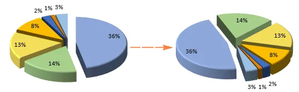

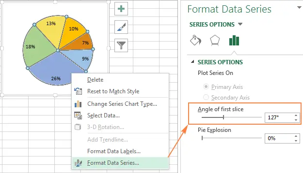
To rotate a pie chart in Excel, follow these steps:

1. Right-click on any sector of the diagram and select the item from the drop-down menu “Data Series Format”.
2. In the side menu that opens, find the section “Row Options”, and in it – the slider “Angle of rotation of the first sector”. Move the slider to rotate clockwise or counterclockwise, or manually enter the desired percentage.

Rotation of XNUMXD charts

3D charts have more rotation features than XNUMXD charts. To access the rotation menu, right-click on the diagram and select “Rotation of a three-dimensional figure”.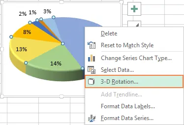

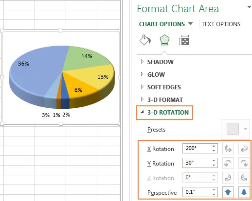
This action will bring up the side menu “Format of a three-dimensional figure” with the following features:

• Rotation along the X and Y coordinate axes.
• Perspective adjustment.

It’s important: XNUMXD charts can be rotated on the X and Y axis, but not on the Z axis. Therefore, you cannot set an arbitrary value for the Z axis manually.

When you click on the up and down arrows located opposite the degree values, the Excel chart will rotate in accordance with the changes made. Therefore, if you are not sure what exact rotation value to set, click the arrows until you give the diagram the optimal position.

Sorting chart fragments by size

Pie charts become easier to read if the sectors in them are arranged in order from wide to narrow. If it is not possible to distribute sectors in descending order, then you can do it manually as follows:

1. Create a pivot table (how to do this, see the corresponding guide on our website).
2. Enter names in “Line Names”, and numerical data – in “Values”. The resulting table will look like this:

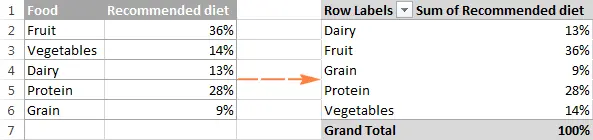
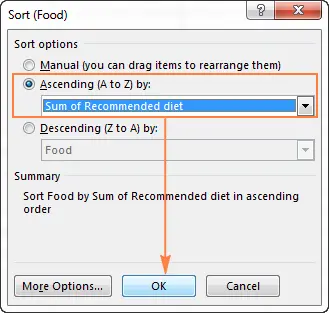
3. Нажмите кнопку “Auto sort” opposite the field “Line Names”, and then select “Additional sorting options”.
4. In the window that opens, select sorting data in descending or ascending order:

5. Create a new chart based on the PivotTable.

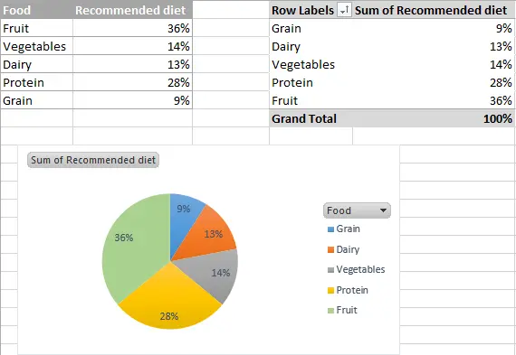
Chart color palette

If for any reason you are unhappy with the coloring of the resulting pie chart, there are two ways to fix it.

Change the color palette of an entire chart

Select a new color theme by clicking “Style…” to the right of the graph. Go to the tab “Color” and apply any theme you like.

Alternatively, click on an arbitrary fragment of the chart to activate the tab “Working with charts” in the toolbar. Go to tab “Constructor” and find the panel “Chart Styles”. To the left of it is a tool “Change Colors”: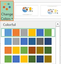

Color selection for individual fragments

As you can see from the screenshot above, Excel offers a rather limited selection of color themes. Therefore, if you want to make your chart as informative and attractive as possible, a good solution would be to manually color each sector. In addition, this approach will be justified when you need to place labels inside chart fragments.

To change the hue of a particular sector, double-click on it to select it, go to the tab “Format”, find there “shape fill” and select the desired shade: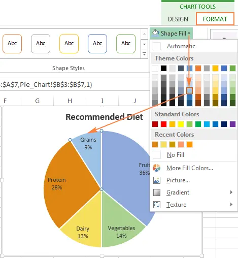

Council: If the graph includes several narrow slices, then mark them with shades of gray to emphasize their insignificance relative to large sectors.

Layout of pie charts

Before using graphs in presentations or exporting to third-party programs, they should be brought to the most presentable form.

To go to the formatting tools, right-click on an arbitrary fragment of the chart and select “Data Series Format”. In the side menu, go to “Effects” (second in a row). There, play with the settings for the shadow, anti-aliasing and relief of the shape.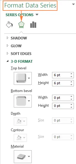

More formatting tools are available on the Format tab:

• Width and height adjustment.
• Fill.
• Shape effects (shadow, relief, etc.).

To use the formatting tools, select the desired fragment of the chart and go to the tab “Format”. Applicable tools are activated automatically, while inactive ones are greyed out.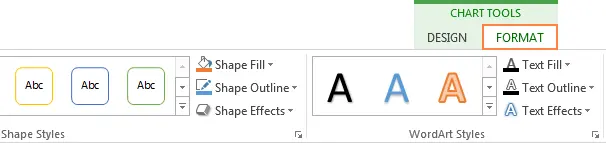

Let’s summarize the basic yes’s and no’s that will help your charts look as informative and presentable as possible.

• • Sort graph fragments by size. To make the information easier to perceive, arrange the sectors from largest to smallest.

• Group elements. If the graph consists of many small sectors, combine them into meaningful groups, and also use colors of similar shades to indicate them.

• • Color minor fragments in gray. If the graph includes several sectors that occupy 2% of the total area or less, then combine them into one “gray” category (as an option, by marking it “Other”).
  • Rotate Chart so that small sectors are in the foreground.

• Don’t use too many categories. This will turn the graph into an unreadable mess. If you have more than 7 categories, draw an auxiliary chart and move all the narrow fragments of the chart into it.

• Get rid of the legend. Instead, label the categories directly on the sectors of the graph so that it is easy to read without having to constantly refer to the legend.
• Don’t overuse effects. An excess of “beautiful” effects significantly reduces the information content of the graph.

Congratulations, now you can draw pie charts of any complexity! In the next part of the tutorial, we will look at working with histograms. Thanks for reading, and see you soon!