How to Create a Waterfall Chart in Excel

Contents

What is a waterfall chart?
How to build a waterfall chart (Bridge, Waterfall) in Excel?

If you use Excel frequently, you probably know firsthand the benefits of charts. Graphical representation of data is very useful when you need to visually compare data or indicate the direction of development.

Microsoft Excel offers many built-in chart types, including bar charts, bar charts, pie charts, and other chart types. In this article, we will take a closer look at all the details of creating the simplest charts, and in addition, we will get to know a special type of chart – waterfall chart in excel (analogue: waterfall diagram). You will learn what a waterfall chart is and how useful it can be. You will learn the secret of creating a waterfall chart in Excel 2010-2013, as well as learn various tools that will help you make such a chart in just a minute.

So, let’s start improving our Excel skills.

Translator’s Note: The waterfall chart has many names. The most popular of them: Waterfall, Bridge, Stupenki и flying bricks, English variants are also common – Waterfall и Bridge.

What is a waterfall chart?

First, let’s see what the simplest Waterfall chart looks like and how it can be useful.

Waterfall diagram is a special type of chart in Excel. Usually used to show how the original data increases or decreases as a result of a series of changes.

The first and last columns in a typical waterfall chart show the total values. Intermediate columns are floating and usually show positive or negative changes occurring from one period to another, and ultimately the overall result, i.e. total value. As a rule, columns are colored in different colors to clearly highlight positive and negative values. Later in this article, we will talk about how to make intermediate columns “float”.

The waterfall chart is also called “Bridge“because floating columns create a kind of bridge connecting extreme values.

These charts are very convenient for analytical purposes. Whether you want to evaluate a company’s profit or product revenue, analyze sales, or simply see how your Facebook friend count has changed over the year, an Excel waterfall chart is the way to go.

How to build a waterfall chart (Bridge, Waterfall) in Excel?

Don’t waste time looking for a waterfall chart in Excel – it’s not there. The problem is that there is simply no ready-made template for such a chart in Excel. However, it’s not difficult to create your own chart by organizing your data and using Excel’s built-in stacked bar chart.

Translator’s Note: In Excel 2016, Microsoft has finally added new chart types, and among them you will find the Waterfall chart.

For a better understanding, let’s create a simple table with positive and negative values. Let’s take sales volume as an example. From the table below, it can be seen that over the course of several months, sales rose and then fell relative to the initial level.

The Bridge chart in Excel will perfectly show the fluctuations in sales over a given twelve months. If you now apply a stacked histogram to these specific values, then nothing like a waterfall chart will work. Therefore, the first thing to do is carefully reorder the existing data.

Step 1. Change the order of the data in the table

First of all, let’s add three additional columns to the original table in Excel. Let’s call them Base, Fall и Rise. Column Base will contain the calculated initial value for the segments of the decline (Fall) and growth (Rise) on the diagram. All negative fluctuations in sales volume from the column Sales Flow will be placed in a column Fall, and positive – in the column Rise.

Also I added a line called End below the list of months to calculate the total sales for the year. In the next step, we will fill in these columns with the desired values.

Step 2. Insert formulas

The best way to fill a table is to paste the desired formulas into the first cells of the respective columns and then copy them down into adjacent cells using the autofill handle.

Selecting a cell C4 in a column Fall and paste in the following formula:
=IF(E4<=0,-E4,0)
=ЕСЛИ(E4<=0;-E4;0)
The meaning of this formula is that if the value in the cell E4 less than or equal to zero, a negative value will be shown as positive, and zero will be shown instead of a positive value.

Note: If you want all values in the waterfall chart to lie above zero, then you must enter a minus sign (-) before the second cell reference E4 in the formula. A minus times a minus makes a plus.

Copy the formula down to the end of the table.
Click on a cell D4 and enter the formula:
=IF(E4>0,E4,0)
=ЕСЛИ(E4>0;E4;0)
This means that if the value in the cell E4 greater than zero, then all positive numbers will be displayed as positive, and negative - as zero.
Use the autofill handle to copy this formula down the column.
Paste the last formula into a cell B5 and copy it down, including the line End:
=B4+D4-C5
This formula calculates the initial values that will raise the rise and fall bars to their respective heights on the chart.

Step 3: Create a Standard Stacked Histogram

Now all the necessary data has been calculated, and we are ready to start plotting the chart:

Highlight data including row and column headers except column Sales Flow.
Click the tab Insert (Insert), find the section Diagrams (Charts).
Click Insertis a histogram (Insert Column Chart) and from the drop down menu select Stacked bar chart (Stacked Column).

A chart will appear that still bears little resemblance to a waterfall chart. Our next task is to turn the Stacked Bar Chart into a Waterfall Chart in Excel.

Step 4: Converting a Stacked Histogram to a Waterfall Chart

It's time to reveal the secret. In order to convert a stacked bar chart to a waterfall chart, you just need to make the values of the data series Base invisible on the chart.

Highlighting a series of data on a chart Base, right-click on it and select from the context menu Data series format (Format data series).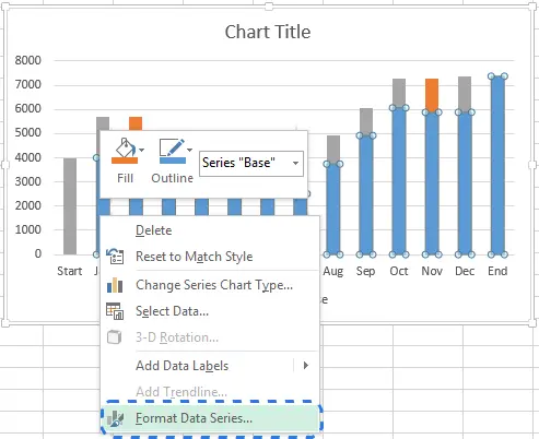In Excel 2013, a bar will appear on the right side of the worksheet Data series format (Format Data Series).
Click on the icon Shading and Borders (Fill & Line).
In section Accordinglivka (Fill) select No fill (No fill), in section Border (Border) – no lines (No line).

After the blue columns have become invisible, all that remains is to delete Base from the legend so that there is no trace of this data series on the chart.

Step 5. Set up a waterfall chart in Excel

Finally, let's do some formatting. First, I'll make the floating blocks brighter and highlight the initial (Home) and final (End) values on the chart.

Selecting a series of data Fall on the diagram and open the tab Framework (Format) in the tab group Working with charts (Chart Tools).
In section Shape styles (Shape Styles) click Shape fill (Shape Fill).
In the drop-down menu, select the desired color. Here you can experiment with the outline of the columns or add any special effects. To do this, use the options menu figure outline (Shape Outline) и Shape Effects (Shape Effects) tab Framework (Format). Next, we will do the same with a series of data Rise. Regarding columns Home и End, then you need to choose a special color for them, and these two columns should be colored the same. As a result, the chart will look something like this:

Note: Another way to change the shading and outline of columns in a chart is to open the panel Data series format (Format Data Series) or right-click on the column and select options in the menu that appears Fill (Fill) or Circuit (Outline).

You can then remove the extra spacing between the columns to bring them closer together.
Double click on one of the chart columns to bring up the panel Data series format (Format Data Series)
Set for parameter Side clearance (Gap Width) small value, e.g. 15%. Close the panel.There are no unnecessary gaps in the Waterfall chart now.
Looking at the waterfall chart, it may seem that some blocks are the same size. However, if you go back to the original datasheet, you can see that the values are not the same. For a more accurate analysis, it is recommended to add labels to the chart columns.
Select the data series to which you want to add labels.
Right-click and select from the context menu that appears. Add data labels (Add Data Labels).Do the same for the other columns. You can adjust the font, text color, and label position to make them easier to read.

Note: If the difference between the sizes of the columns is obvious, and the exact values of the data points are not so important, then the labels can be removed, but then the y-axis should be shown to make the chart clearer.

When you're done with the column labels, you can get rid of unnecessary elements, such as zero values and the chart legend. In addition, you can think of a more descriptive title for the chart. How to add a title to a chart in Excel is described in detail in one of the previous articles.

The waterfall chart is ready! It differs significantly from the usual types of diagrams and is extremely clear, isn't it?

Now you can create a whole collection of waterfall charts in Excel. I hope it won't be difficult for you. Thank you for your attention!