How to Create a Pareto Chart in Excel

The Pareto chart combines a bar chart and a line chart. The Pareto principle states that the following statement is true for many cases: 20% of efforts give about 80% of results. In this example, we will see that 80% of all complaints are complaints of two types out of ten possible, which corresponds to 20%.

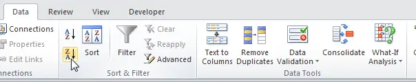
1. First of all, sort the data in the cells in descending order. To do this, left-click on the top cell in the column Count (number of complaints), then on the tab Data (Data) find and click the button ЯА (ZA) – descending sort.
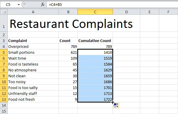
2. Next, let’s calculate the amount with accumulation (Cumulative Count). To do this, enter the following formula in a cell С5 and drag it down the entire column.
3. Next, we calculate the accumulated interest (Cumulative%). To do this, enter the following formula in a cell D4 and drag it down the entire column.

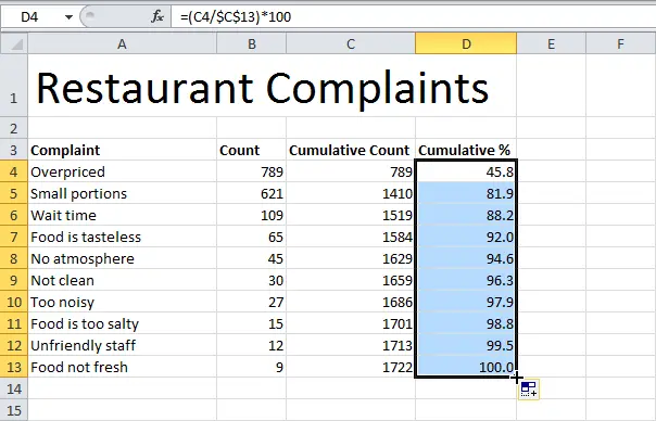
Note: In a cell С13 the total number of complaints is displayed. When dragging a formula down, an absolute reference $C$13 remains unchanged, while the relative С4 changes to C5, C6, C7, etc.

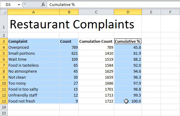
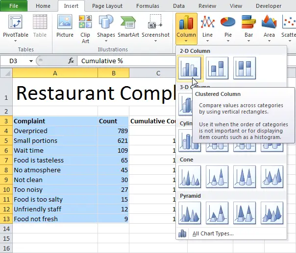
4. Highlight data in columns A, B и D. To do this, press and hold the key Ctrl while selecting the desired range of cells in each column.
5. On the Advanced tab Insert (Insert) click the button bar chart (Column), then from the drop-down menu select Histogram with grouping (Clustered Column).
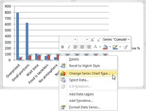
6. Right-click on the red columns (accumulated %) and from the context menu select Change the chart type for a series (Change Series Chart Type).
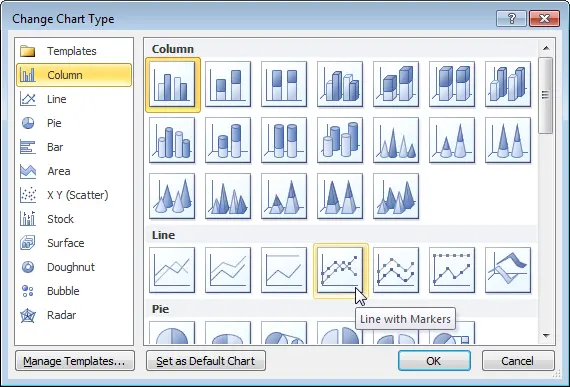
7. Select type Graph with markers (Line with Markers).
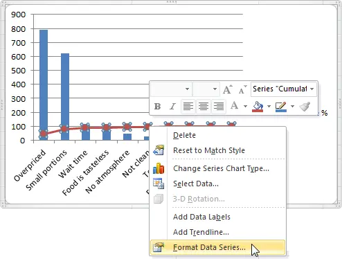
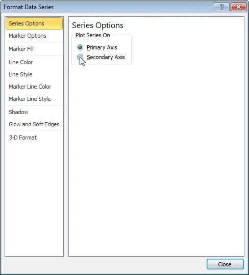
8. Right click on the red line and select Data series format (Format Data Series).
9. Select item Minor Axis (Secondary Axis).
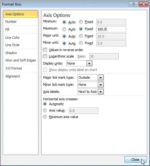
10. Right click on the minor axis (percentage axis) and select Axis Format (Format Axis), set Maximм (Maximum) equal 100 and press Close (Close).

As a result, we get the following:

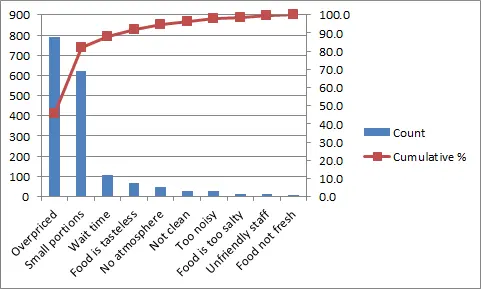
Conclusion: The Pareto chart shows that 80% of all complaints are complaints of 20% of the types: Too expensive (Overpriced) and Small portions (Small portions). In other words, we see the Pareto principle in action.