


If neither cell selection rules, nor rules for selecting first and last values, nor histograms, nor color scales, nor icon sets are sufficient for your task, create your own conditional formatting rule.
As an example, in the figure below, select the codes (column Code) that occur in the range A2: A10 more than once and have a score (Score column) greater than 100.
- Highlight a range A2: A10.
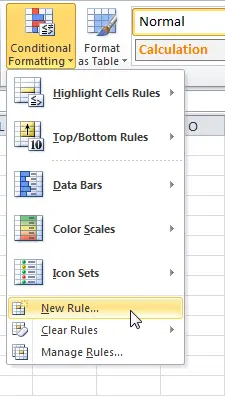
- On the Advanced tab Home (Home) select a team Conditional Formatting > Create Rule (Conditional Formatting > New Rule).

Note: Cell selection rules, first and last selection rules, histograms, color scales, and icon sets can also be included in the new rule.
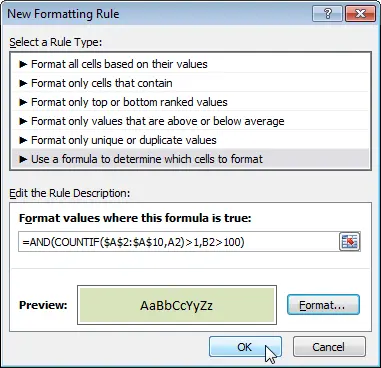
- Click on Use a formula to determine which cells to format (Use a formula to determine which cells to format).
- Enter the following formula:
=AND(COUNTIF($A$2:$A$10,A2)>1,B2>100)=И(СЧЕТЕСЛИ($A$2:$A$10;A2)>1;B2>100) - Select a formatting style and click OK.
 Result: Excel formatted the cell A5because the code А occurs in the range A2: A10 more than once, and the value in the cell B5 more 100.
Explanation:
- The expression COUNTIF($A$2:$A$10,A2) counts the number of codes in the range A2: A10, equal to the code in the cell A2.
- If COUNTIF($A$2:$A$10,A2)>1 and B2>100, Excel formats the cell A2.
- Since we have chosen a range A2: A10 Before using conditional formatting, Excel will automatically copy the formulas to the rest of the cells in the range. So the cell A3 будет содержать формулу:=И(СЧЕТЕСЛИ($A$2:$A$10;A3)>1;B3>100),ячейка A4:
=И(СЧЕТЕСЛИ($A$2:$A$10;A4)>1;B4>100) и т.д.
- Note that we have used an absolute reference − $A$2:$A$10.