How to “color” a cell depending on its value in an Excel spreadsheet

Often, users of a spreadsheet editor face such a task when it is necessary to give a cell a certain color depending on its value on the worksheet. There are many ways to implement this simple procedure. In the article, we will consider in detail all the options that allow you to give a color to a cell depending on its value.

The process of editing colors in a spreadsheet editor

A plate designed so that certain meanings have their own shade allows you to visually and structuredly present information. It is especially important to implement such a procedure in tabular files, which contain a large amount of information. Color shading will allow users to quickly navigate large amounts of data.

Worksheet objects can be “colored” on their own, but this option is not suitable in cases where there is too much information. In addition, when filling manually, you can make several mistakes. There are two automatic ways to fill a cell with color. Let’s consider each method in more detail.

Method One: Using Conditional Formatting

Conditional formatting allows you to specify specific measure boundaries at which worksheet fields will be colored in a certain color. “Painting” occurs automatically. If the cell index goes beyond the border, then the repainting of this worksheet object is automatically implemented.

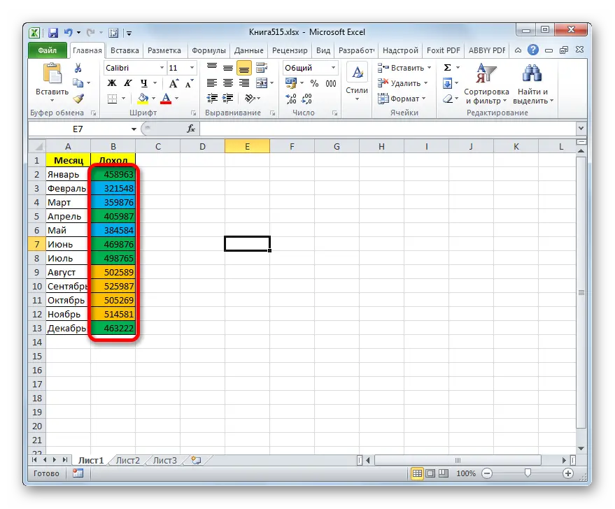
Let’s consider the work of this method on a specific example. For example, we have a table that displays the monthly profit of a certain organization. Purpose: to designate with different colors the elements in which the profit margin is below 400000 rubles, from 400000 to 500000 rubles, and also more than 500000 rubles. Detailed instructions look like this:

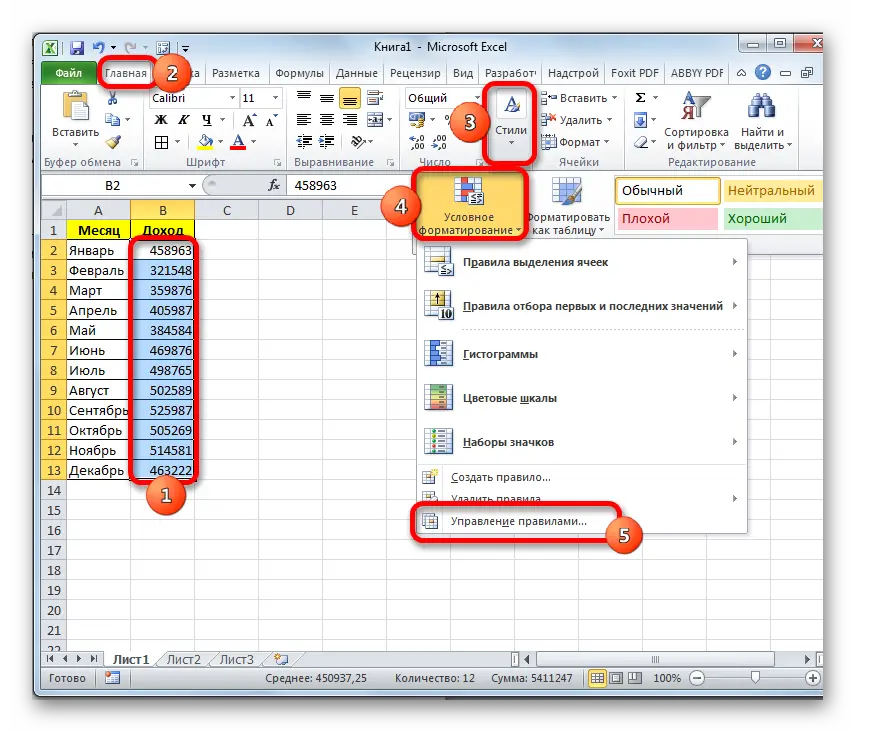
1. We make a selection of the column in which the data on the profit of the organization are located. We move to the “Home” subsection. Click on the “Conditional Formatting” button located in the “Styles” command block. In the drop-down list, click on the element “Manage rules …”.

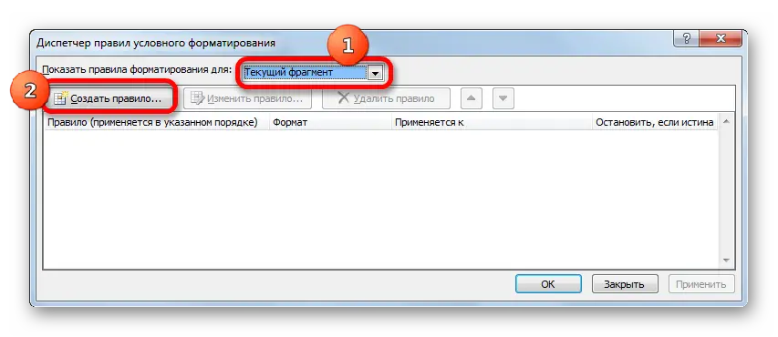
2. A window appeared on the display called Conditional Formatting Rules Manager. In the line “Indicator of the formatting rule for” set the element “Current Fragment”. To confirm the settings made, click on “Create a rule …”.

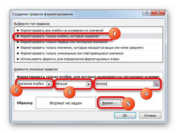
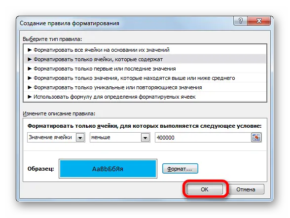
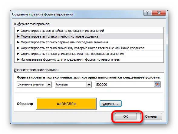
3. A window appeared on the screen with the name “Creating a formatting rule”. In the “Select a rule type:” box, select the “Format only cells that contain” item. In the 1st line, specify the parameter “Values”. In the 2nd line, specify the parameter “Less”. In the 3rd line, we indicate the indicator 400000. To confirm the settings made, click on “Format …”.

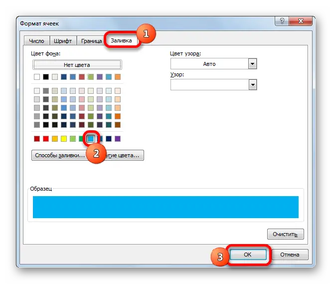
4. A window appeared on the display with the name “Format Cells”. We move to the “Fill” subsection. We select the shade that we plan to set for cells with indicators less than 400000. To confirm the settings made, click on “OK”.

5. We return to the previous window and click on “OK”.

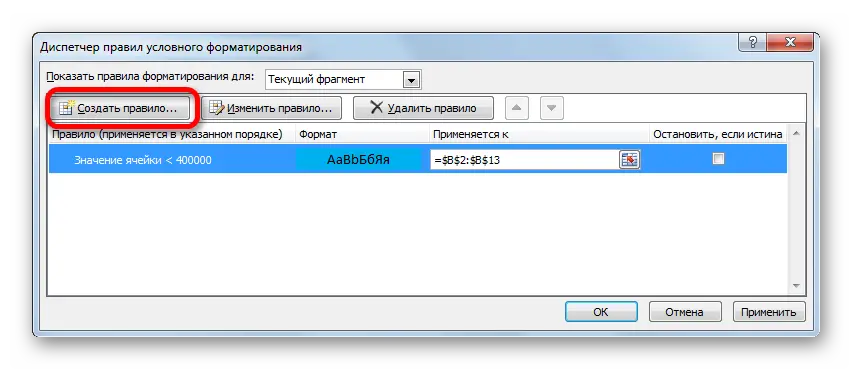
6. We ended up in the “Conditional Formatting Rules Manager” window again. We added a rule we created here. Once again, click on the “Create Rule …” element.

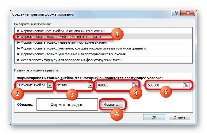
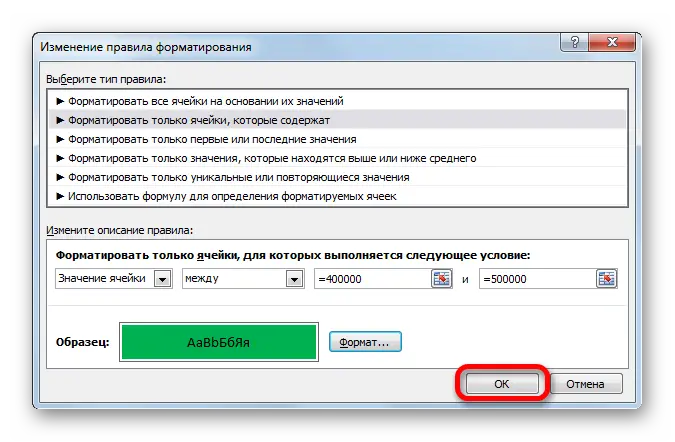
7. A window with the name “Creating a formatting rule” appeared again on the screen. In the “Select a rule type:” box, select the “Format only cells that contain” item. In the 1st line, specify the parameter “Values”. In the 2nd line, specify the parameter “Between”. In the 3rd line we indicate the indicator 400000. In the 4th line we indicate the value 500000. To confirm the settings made, click on “Format …”.

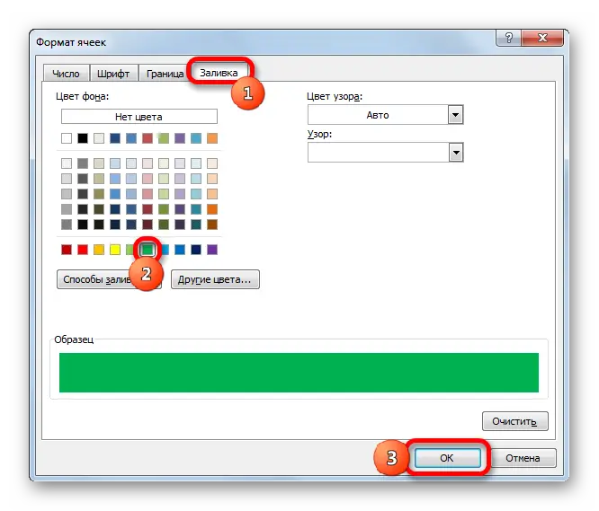
8. A window appeared on the display with the name “Format Cells”. We move to the “Fill” subsection. We select a different shade, which we plan to set to cells with indicators between 400000 and 500000. To confirm the settings made, click on “OK”.

9. We return to the previous window and click on “OK”.

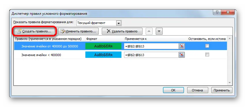
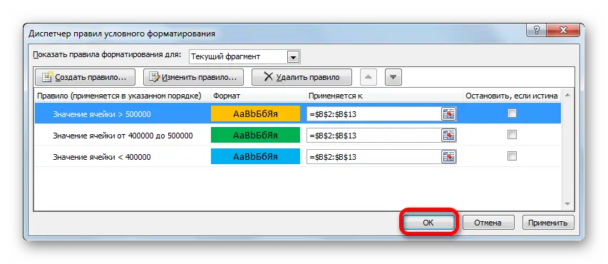
10. In the “Conditional Formatting Rules Manager” window, we already have 2 rules created. It remains to add one more thing. Once again, click on the “Create Rule …” element.

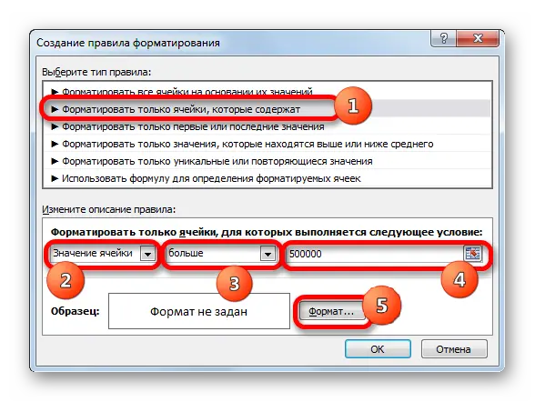
11. A window with the name “Creating a formatting rule” appeared again on the screen. In the “Select a rule type:” box, select the “Format only cells that contain” item. In the 1st line, specify the parameter “Values”. In the 2nd line, specify the parameter “greater than”. In the 3rd line, we indicate the indicator 500000. To confirm the settings made, click on “Format …”.

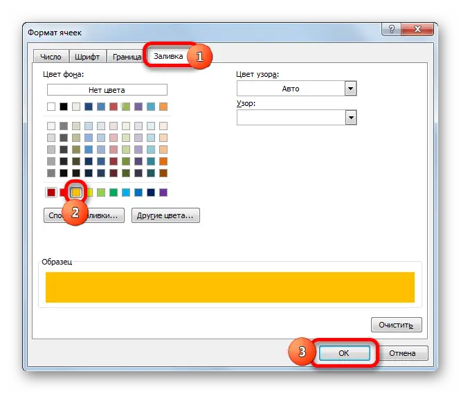
12. A window appeared on the display with the name “Format Cells”. We move to the “Fill” subsection. We select a different shade, different from the previous two, which we plan to set to cells with indicators greater than 500000. To confirm the settings made, click on “OK”.

13. We return to the previous window and click on “OK”.

14. We have created three rules. We click on “OK”.

15. Ready! We implemented coloring according to the specified rules.

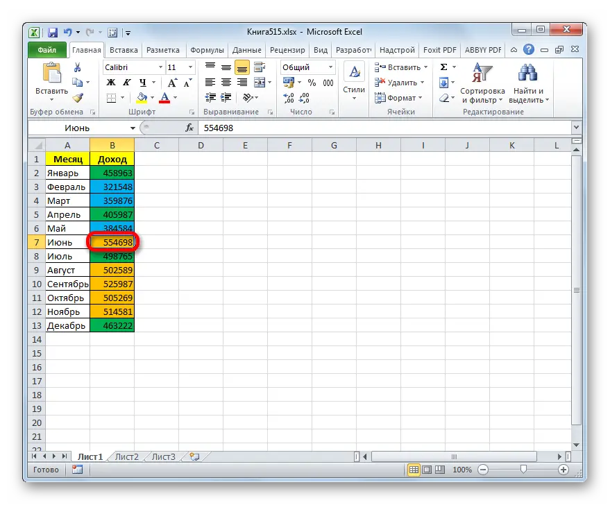
If you edit the content of any cell, going beyond the 1st of the specified rules, then the cell will change its shade on its own.

Method Two: An Additional Variation of Using Conditional Formatting

Using conditional formatting, you can implement coloring in another way. Detailed instructions look like this:

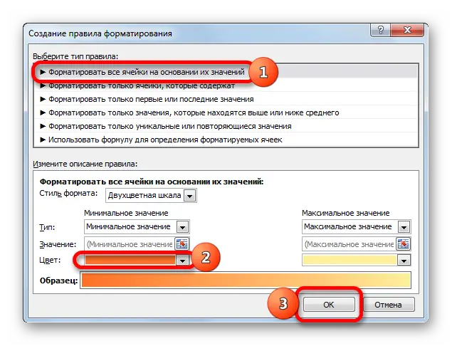
1. Once in the window called “Create a formatting rule”, select the element “Format cells based on their values.” In the “Color” line, select the shade with which we plan to color the worksheet objects. We click on “OK”.

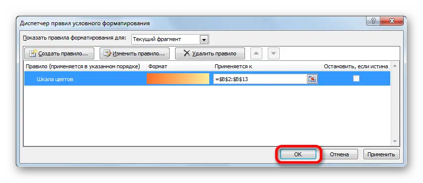
2. In the Rules Manager window, click OK.

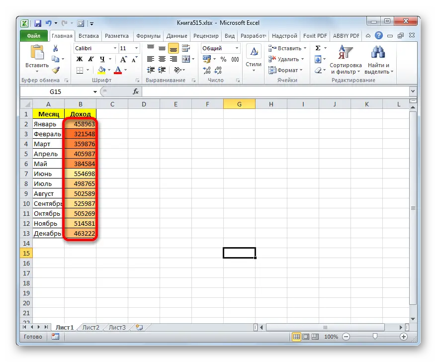
3. As a result of the actions taken, the cells of the selected column were painted with various shades of the selected color. Higher values ​​are colored in lighter shades, and smaller values ​​are colored in darker ones.

Conclusion and conclusions about coloring cells depending on the values

We found out that there are several ways to color cells depending on the values. All actions are carried out using conditional formatting. Each user can independently choose the most convenient method for himself.