How to change the color of a row in Excel depending on the value in a cell

Contents

How to change the color of a row based on the numeric value of one of the cells
How to create multiple conditional formatting rules with a given priority
How to change the color of a row based on the text value of one of the cells
How to change the color of a cell based on the value of another cell
How to set multiple conditions to change the color of a row

Learn how to quickly change the color of an entire row in Excel sheets based on the value of a single cell. See tricks and examples of formulas for numeric and text values.

In one of the previous articles, we discussed how to change the color of a cell depending on its value. This time we will talk about how to highlight the entire row in Excel 2010 and 2013 depending on the value of one cell, and also reveal a few tricks and show examples of formulas for working with numeric and text values.

How to change the color of a row based on the numeric value of one of the cells

Suppose we have the following table of company orders:

We want to color the rows with different colors depending on the quantity ordered (the value in the column Qty.) to highlight the most important orders. The Excel tool will help us to cope with this task – “Conditional Formatting».

First of all, select all the cells whose fill color we want to change.
To create a new formatting rule, click Home > Conditional Formatting > Create Rule (Home > Conditional Formatting > New rule).
In the dialog box that appears Create a formatting rule (New Formatting Rule) select the option Use a formula to determine which cells to format (Use a formula to determine which cells to format), and below, in the field Format values for which the following formula is true (Format values where this formula is true), enter the following expression:
=$C2>4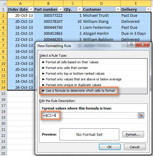
Instead of C2 You can enter a link to another cell in your table whose value you want to use to test the condition, and instead of 4 you can enter any number you want. Of course, depending on the task, you can use the comparison operators less than (<) or equal to (=), that is, write the formulas in this form:
=$C2<4
=$C2=4
Notice the dollar sign $ before the cell address - it is needed in order to keep the column letter unchanged when copying the formula to the remaining cells of the row. Actually, this is the secret of focus, which is why the formatting of the entire row changes depending on the value of one given cell.
Push the button Framework (Format) and go to the tab Fill (Fill) to select the background color of the cells. If the standard colors are not enough, click the button Other colors (More Colors), choose the appropriate one and double click OK.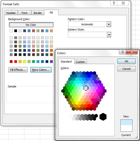In the same way on the other tabs of the dialog box Cell format (Format Cells) other formatting options are configured, such as font color or cell borders.
In the Sample (Preview) shows the result of executing the created conditional formatting rule:
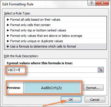
If everything turned out as planned, and the selected color suits you, then click OKto see the created rule in action. Now, if the value in the column Qty. more 4, then the entire row of the table will turn blue.

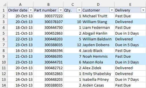
As you can see, changing the color of an entire row in Excel based on the numerical value of one of the cells is not at all difficult. Next, we will look at a few more examples of formulas and a couple of tricks for solving more complex problems.

How to create multiple conditional formatting rules with a given priority

In the table from the previous example, it would probably be more convenient to use different fill colors to highlight the rows containing in the column Qty. different values. For example, create another conditional formatting rule for strings containing the value 10 or more, and highlight them in pink. For this we need a formula:

=$C2>9

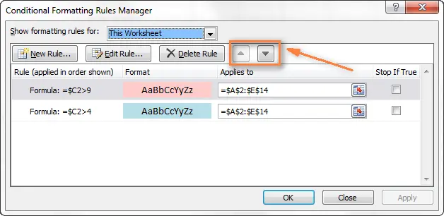
In order for both rules we created to work simultaneously, you need to arrange them in the right priority.

On the Advanced tab Home (Home) section Styles (Styles) click Conditional Formatting (Conditional Formatting) > Rule management (Manage Rules)
In the dropdown list Show formatting rules for (Show formatting rules for) select This sheet (This worksheet). If you want to change the settings only for the rules on the selection, select the option current fragment (Current Selection).
Select the formatting rule that should be applied first and use the arrows to move it to the top of the list. It should turn out like this:Press OK, and the lines in the specified fragment will immediately change color, in accordance with the formulas in both rules.

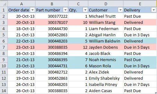
How to change the color of a row based on the text value of one of the cells

To simplify order fulfillment control, we can highlight in our table rows of orders with different delivery statuses with different colors, information about which is contained in the column Delivery:

If the delivery date of the order is in the future (value Due in X Days), then the fill of such cells should be orange;
If the order has been delivered (value Delivered), then the fill of such cells should be green;
If the delivery date of the order is in the past (value Past Due), then the fill of such cells should be red.

And, of course, the cell fill color should change if the order status changes.

With formula for values Delivered и Past Due everything is clear, it will be similar to the formula from our first example:

=$E2="Delivered"

=$E2="Past Due"

The task sounds more difficult for orders that must be delivered through Х days (value Due in X Days). We see that the delivery time for various orders is 1, 3, 5 or more days, which means that the above formula does not apply here, as it is aimed at an exact value.

In this case, it is convenient to use the function SEARCH (SEARCH) and to find a partial match, write the following formula:

=ПОИСК("Due in";$E2)>0

=SEARCH("Due in",$E2)>0

In this formula E2 - this is the address of the cell, based on the value of which we will apply the conditional formatting rule; dollar sign $ needed in order to apply the formula to the whole line; condition ">0" means that the formatting rule will be applied if the specified text (in our case, "Due in") is found.

Tip: If the formula uses the condition ">0“, then the line will be highlighted in color every time the specified text is found in the key cell, regardless of where it is located in the cell. In the example table in the figure below, the column Delivery (column F) may contain the text "Urgent, Due in 6 Hours" (which means - Urgent, deliver within 6 hours), and this line will also be colored.

In order to highlight with color those lines in which the contents of the key cell begin with the specified text or symbols, the formula must be written in the following form:

=ПОИСК("Due in";$E2)=1

=SEARCH("Due in",$E2)=1

You need to be very careful when using such a formula and check if the cells of the key column of data start with a space. Otherwise, you can rack your brains for a long time, trying to understand why the formula does not work.

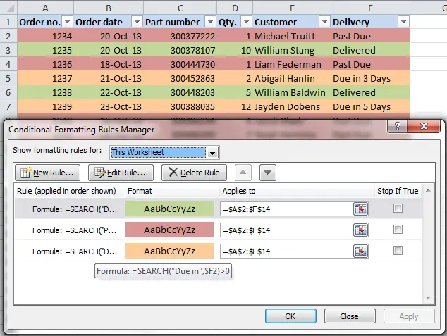
So, following the same steps as in the first example, we created three formatting rules, and our table began to look like this:

How to change the color of a cell based on the value of another cell

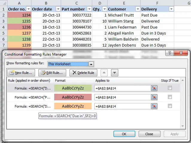
In fact, this is a special case of the task of changing the color of a line. Instead of the whole table, select the column or range in which you want to change the color of the cells, and use the formulas described above.

For example, we can set up three of our rules in such a way that only cells containing an order number are highlighted in color (column Order number) based on the value of another cell in this row (using the values from the column Delivery).

How to set multiple conditions to change the color of a row

If you need to highlight rows with the same color when one of several different values appears, then instead of creating several formatting rules, you can use the functions И (AND), OR (OR) and thus combine several conditions in one rule.

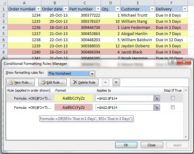
For example, we can mark orders expected within 1 and 3 days in pink, and those due within 5 and 7 days in yellow. The formulas will look like this:

=ИЛИ($F2="Due in 1 Days";$F2="Due in 3 Days")

=OR($F2="Due in 1 Days",$F2="Due in 3 Days")

=ИЛИ($F2="Due in 5 Days";$F2="Due in 7 Days")

=OR($F2="Due in 5 Days",$F2="Due in 7 Days")

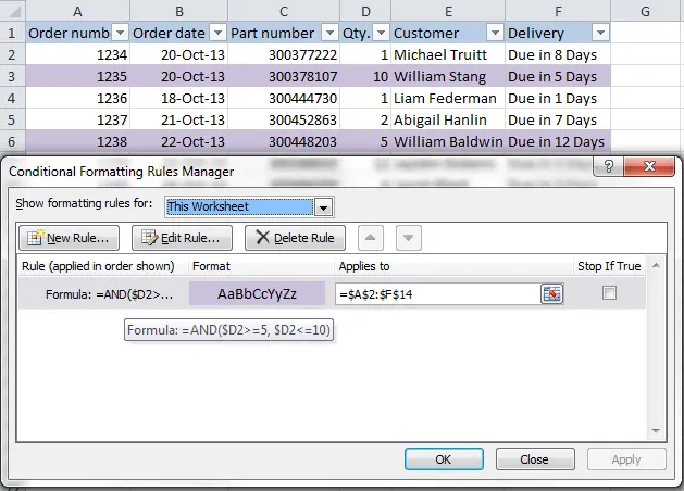
In order to highlight orders with a quantity of at least 5, but not more than 10 items (the value in the column Qty.), write the formula with the function И (AND):

=И($D2>=5;$D2<=10)

=AND($D2>=5,$D2<=10)

Of course, in your formulas you can use not necessarily two, but as many conditions as required. For example:

=ИЛИ($F2="Due in 1 Days";$F2="Due in 3 Days";$F2="Due in 5 Days")

=OR($F2="Due in 1 Days",$F2="Due in 3 Days",$F2="Due in 5 Days")

Tip: Now that you have learned how to color cells in different colors, depending on the values they contain, you may want to find out how many cells are highlighted in a particular color, and calculate the sum of the values in these cells. I want to please you, this action can also be done automatically, and we will show the solution to this problem in an article devoted to the question of How to calculate the amount, amount in Excel and set up a filter for cells of a certain color.

We have shown just a few of the possible ways to make a table look like a zebra stripe, the color of which depends on the values in the cells and can change along with changing these values. If you are looking for something different for your data, let us know and together we will definitely come up with something.