How to Change Series Labels in an Excel Table

Often, when working in the Excel spreadsheet editor, users are faced with such a task as changing the caption of a row in a table. This procedure can be carried out in several ways. In the article, we will analyze in detail all the ways that allow you to edit the labels of a series in a spreadsheet document.

Row arrangement in spreadsheet editor

When a user adds a chart to a spreadsheet document worksheet, its axes remain unlabeled. There are 3 variations of the location of the signature:

1. Rotated.
2. Vertical.
3. Horizontal.

To select the type of signature, you need to perform several actions. Detailed instructions look like this:

1. Open the element “Working with charts”.
2. We move to the “Layout” subsection, which is located at the top of the spreadsheet editor interface. You just need to click the left mouse button on the element itself.
3. We click on the button that has the name “Name of the axes”.
4. A list of two items was revealed: “Primary Horizontal Axis Title” and “Primary Vertical Axis Title”.
5. Having expanded one of the two given elements, you can select the following types: “Rotated title”, “Vertical title”, “Horizontal title”.
6. It is necessary to simply click on the LMB to select the appropriate option. The signature will immediately appear near the row.
7. If you click the left mouse button on the name that appears, you can edit it.
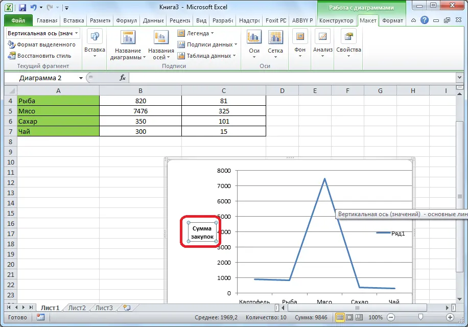
8. The horizontal label looks like this:

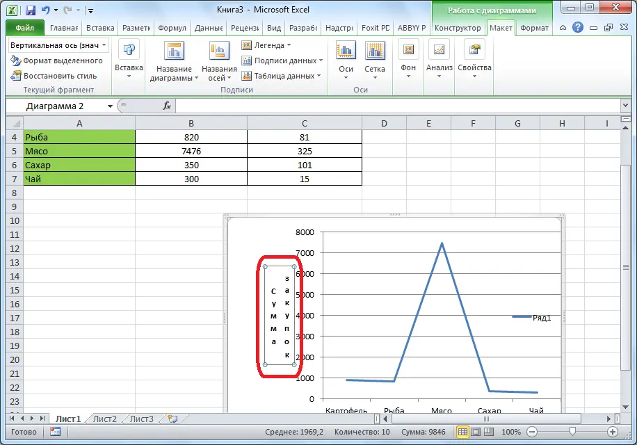
9. The vertical signature looks like this:

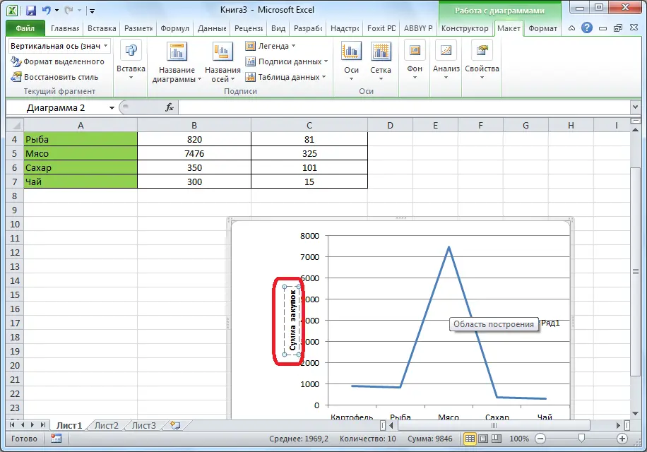
10. The rotated signature looks like this:

It is worth noting that you can additionally edit the size of data labels. To implement this simple procedure, you need to left-click on the data signature, and then stretch its boundaries to the desired size.

Important! Each user of the spreadsheet editor can change the settings and other size and alignment options. To carry out this procedure, it is necessary to double-click the LMB on the data signature itself, and then click on the element named “Size and Properties”. Here you can edit various parameters.

Editing the horizontal row label in the table editor

In addition to the general name, you can edit the name of the values ​​of each element of the series. There are several different changes that can be implemented using the Excel spreadsheet editor. Detailed instructions for editing a horizontal signature look like this:

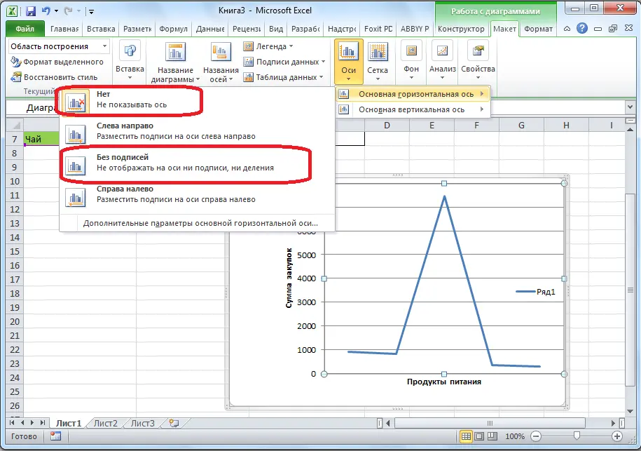
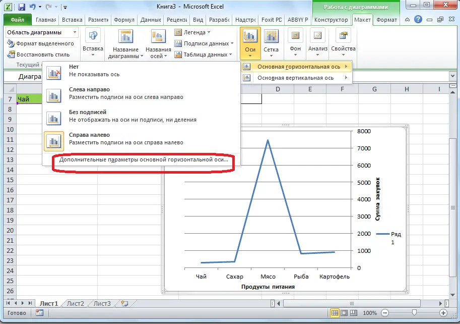
1. To edit the type of axis label of the horizontal type, left-click on the button with the name “Axes”. Expand the list of the element “Main horizontal axis”. By default, the signature is arranged from left to right.. If you click on the element “No labels” or “No”, then they can be completely turned off on the horizontal type axis.

2. If you click the left mouse button on the element that has the name “Right to Left”, then the signature will change its own direction.

3. In addition, you can left-click on the “Additional parameters of the main horizontal axis …”.

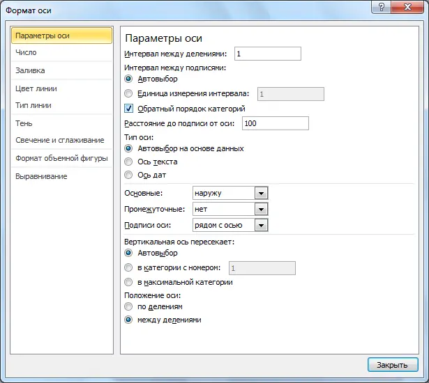
4. A window appeared on the display called “Axis Format” with many different settings. Here you can make detailed settings for the display of the axis. You can set the interval between values, specify the shade of the line, select the format of the label values ​​(text, percentage, monetary, and so on), the type of line, perform alignment, and many other useful settings.

5. Using all these settings, each user can implement a change in the label of a series on a horizontal axis.

Editing the vertical label of a row in the table editor

Now we will analyze in detail how to edit the vertical label of a row in the Excel spreadsheet editor. Detailed instructions for editing a vertical signature look like this:

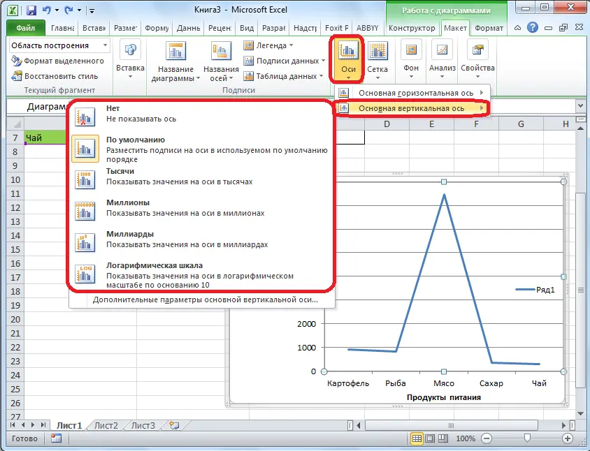
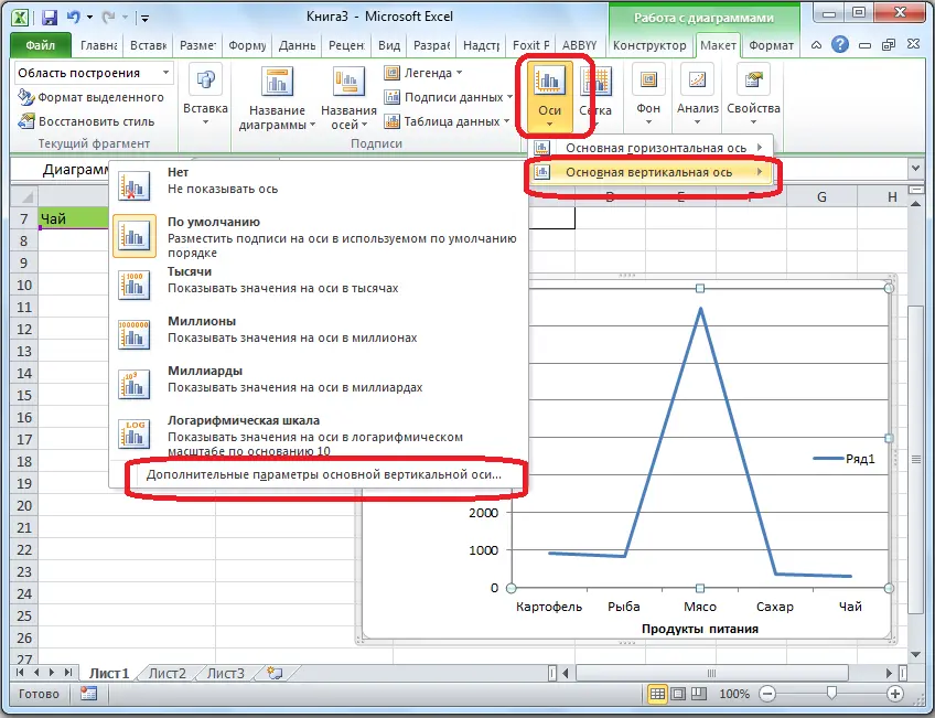
1. To edit the type of vertical type axis label, left-click on the button with the name “Axes”. Expand the list of the element “Primary vertical axis”. If you click on the element “No labels” or “No”, then they can be completely turned off on the horizontal type axis. There are four options for displaying values: “Thousands”, “Millions”, “Billions” and “Logarithmic Scale”.

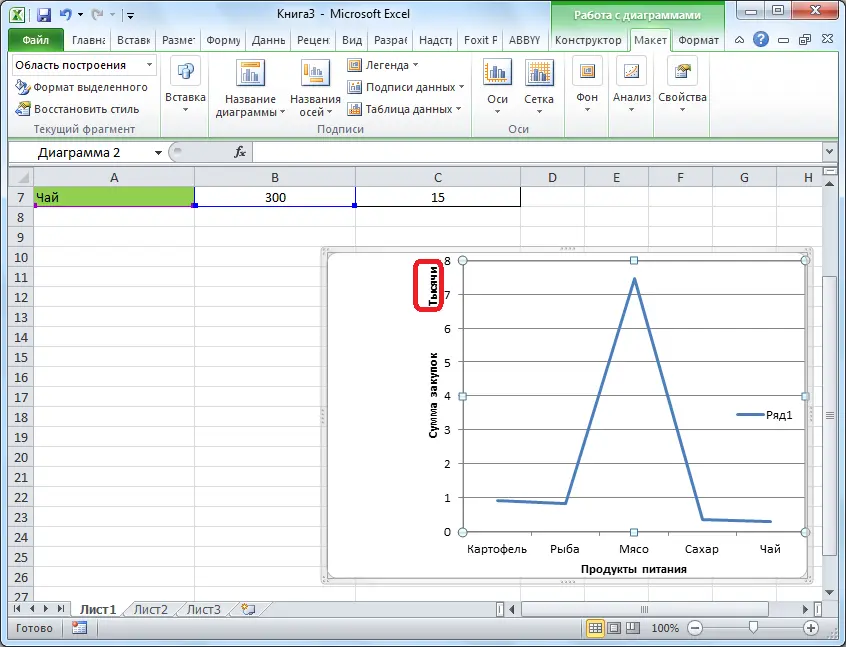
2. In the figure below, you can clearly see how, after selecting one or another display option, the indicators of a row of a vertical type axis are edited.

3. In addition, you can left-click on the “Additional parameters of the main horizontal axis …”.

4. A window appeared on the display called “Axis Format” with many different settings. Here, as in the previous considered option, you can make detailed settings for the display of the axis. You can set the interval between values, specify the shade of the line, select the format of the label values ​​(text, percentage, monetary, and so on), the type of line, perform alignment, and many other useful settings.
5. Using all these settings, each user can implement a change in the label of a series on a vertical type axis.

Conclusion and conclusions about changing the row label in the spreadsheet editor

We found out that there are many ways to edit the labels of a number of vertical and horizontal axes. This procedure is implemented using the elements located on the tool ribbon, which can be found at the top of the spreadsheet editor interface. A variety of additional settings can be set using a special window called “Axis Format”. Each user can independently choose for himself the most convenient way to edit the caption of a series in an Excel spreadsheet document.