How to Change Row Names in an Excel Table

After building a chart in Microsoft Office Excel, the elements marked on it by default remain untitled. For example, instead of the names of the columns, the words “Row”, “Row2”, “Row3”, ​​etc. can be indicated. There are several ways to change these names. They will be discussed in this article.

How to change the series name in a chart in Excel

Within the framework of this topic, only the simplest ways to accomplish the task will be considered, which are implemented using the tools built into the program. Each method deserves detailed study.

Method 1: Using the Chart Tool

The method is extremely simple and is performed intuitively. Even a beginner can handle it. To replace the standard series names and give your own, you can use the following algorithm of actions:

1. Make an initial table and build a chart for specific values.
2. Click with the left mouse button on any place of the plotted graph to select it.
3. Next, you need to move to the “Home” section at the top of the program menu.
4. Find the “Charts” button and expand this subsection by clicking on the arrow next to it.

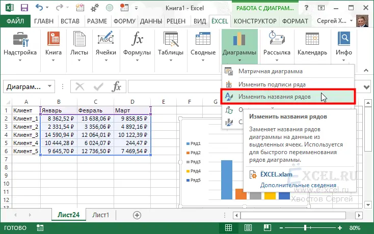
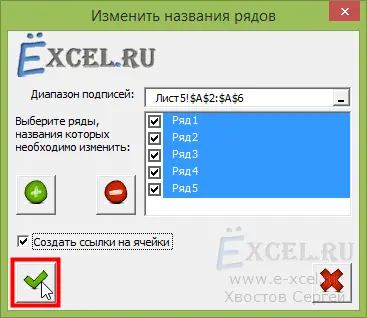
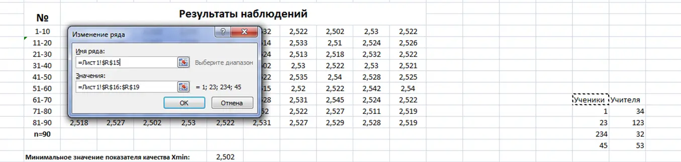
5. In the context menu, click LMB on the line “Change row names”. After that, a special settings window will open, in which the user can give each row a name, indicating the corresponding row in the original table array.
6. When the actions are completed, it remains to click on “OK” at the bottom of the window.

Pay attention! If necessary, this or that series can be hidden from the constructed diagram by unchecking it in the menu for setting the parameters of the series.

Method 2. Changing row names through the “Select data” option

This method is more complicated than the previous one, however, it also needs detailed consideration. To implement it, you need to do the following:

1. Build a chart based on the original table array.
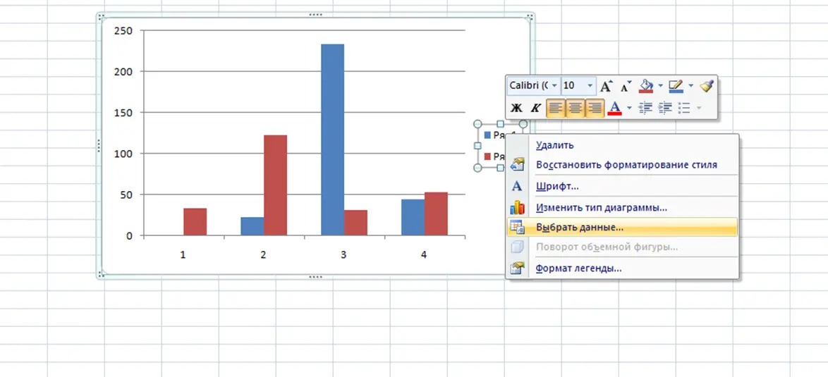
2. Right-click on the name of row 1 in the area of ​​the chart itself.
3. In the context menu that opens, click on the line “Select data …”. This will open another menu.

4. In the “Legend Elements” section, select the desired row, and then click on the “Edit” button.

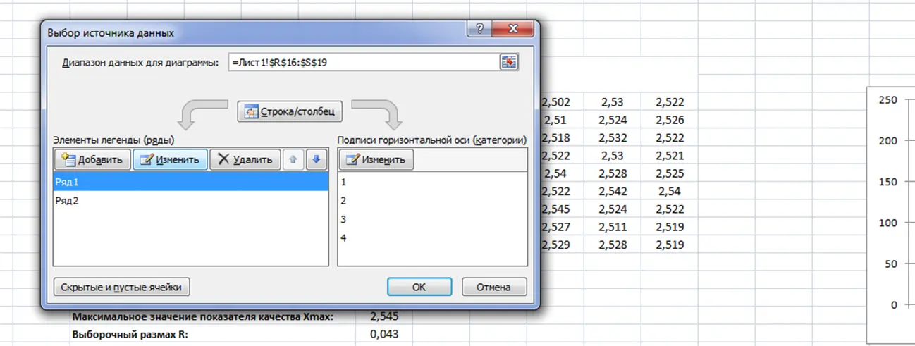
5. In the next window, you need to click on the icon located to the left of the line “Row name”. After this action, Excel will prompt you to select a range of cells in the original table array to give the series a name.
6. Hold LMB and highlight the desired name in the table.

7. Release the left mouse button, check that the first line is filled in the “Change Row” window and click on “OK” to confirm.
8. Check result. The selected row in the chart should be renamed to the value from the original plate.
9. Do the same procedure with the name of the remaining rows of the graph.

Important! The method discussed above takes a lot of time to implement for the PC user, who will have to do the steps to change the name separately for each row. However, the method is relevant, especially if the chart has a small number of series.

How to immediately build a chart with the correct name of the series

If the original table in Excel has a small size and a small number of columns, then the user can immediately create a chart with named series. To implement this possibility, you must act according to the following scheme:

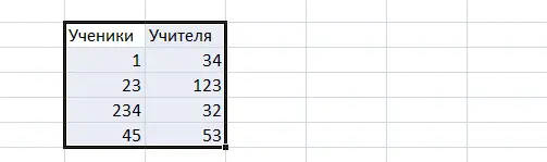
1. Create a table for which you want to build a graph. For example, the array will consist of only two columns.
2. Hold down the left mouse button and select the entire table along with the header. The column headings in the table will subsequently become the names of the series in the diagram.

3. Next, you should move to the “Insert” section, located at the top of the main menu of the Excel program.
4. In the “Charts” area, expand the “Bar” subsection and at the end of the list of suggested options, click on the “All types of charts …” button.
5. Choose any of the bar chart options you like and click OK at the bottom of the window.
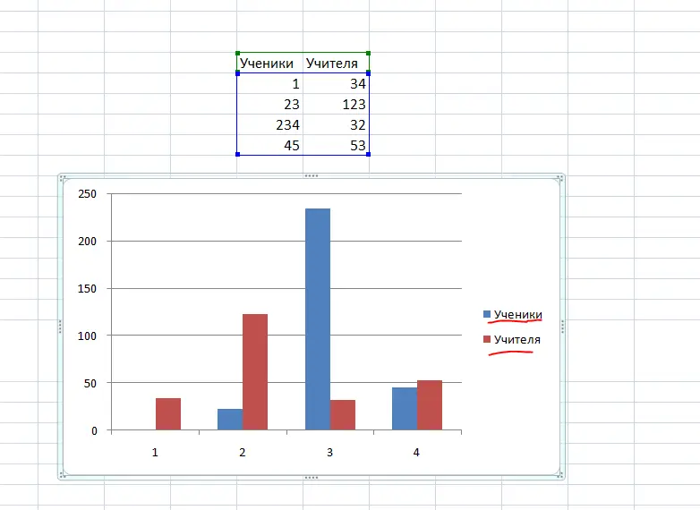
6. The selected graph will be displayed next to the original table array. If desired, it can be stretched or dragged to another place on the program worksheet.
7. Check result. Now the names of the series on the diagram will be written correctly in accordance with the table, and the user will not need to change them using the above methods.

Additional Information! If desired, a name can be added to the constructed diagram. How to do this will be discussed next.

How to name a chart in Excel

Regardless of the software version, the constructed chart can be renamed as follows:

1. Build a diagram and select it with LMB.
2. Enter the “Constructor” section at the top of the MS Excel main menu.
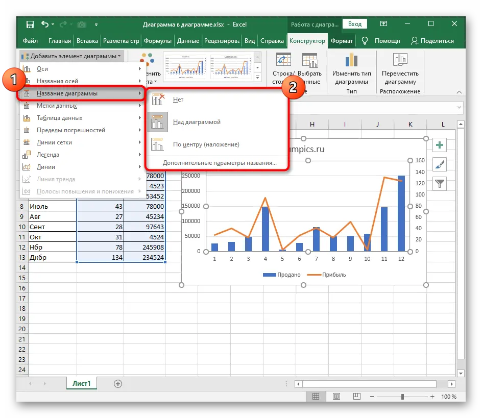
3. Expand the line on the left “Add” a chart element by clicking on the arrow next to it.
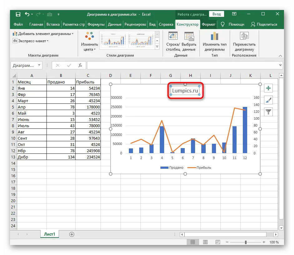
4. In the drop-down menu, you need to move the mouse cursor over the “Chart Name” field and select its location on the chart.

5. Now all that remains is to select the name itself that appears on the chart, double-click on it with LMB and rename it. Here you can write any word, phrase from the PC keyboard.

Conclusion

Thus, in Microsoft Office Excel, you can build any type of chart using a table and quickly set the desired name for the series by selecting the appropriate range of cells in the original array. The main methods for accomplishing the task were discussed above.