


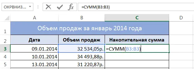
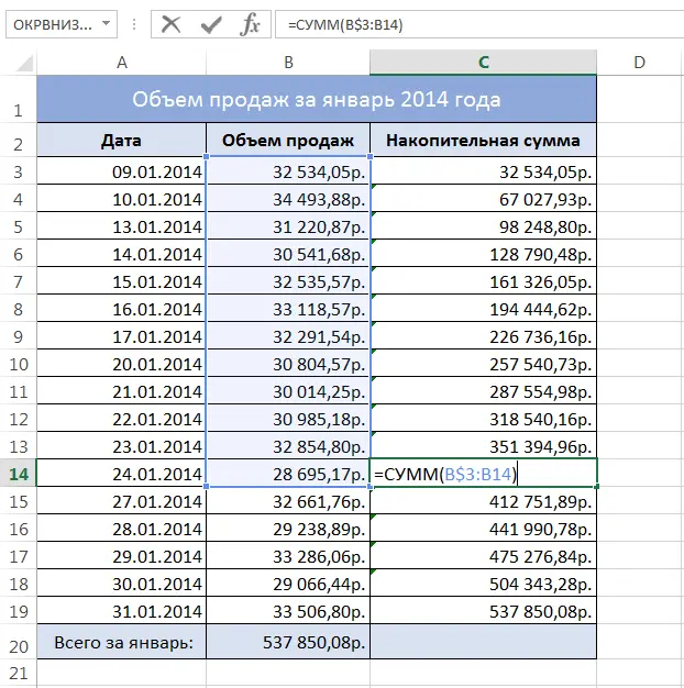
In the figure below you can see an Excel table that shows the sales volume by day for the month of January 2014. Cell B20 shows the total sales for the entire month, calculated using the function SUM. It is required to calculate the sales volume for each date in January relative to the beginning of the month, i.e. cumulative amount.
When calculating the accumulative sum in Excel, it is necessary that the summation always starts from the third row (cell B3) and ends with the row in question. For example, cell C3 should contain the following formula: =SUM(B3), and to be more precise, =SUM(B3:B3), i.e. summation of a range consisting of one cell.
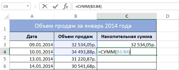
Cell C4 this formula: =SUM(B3:B4)
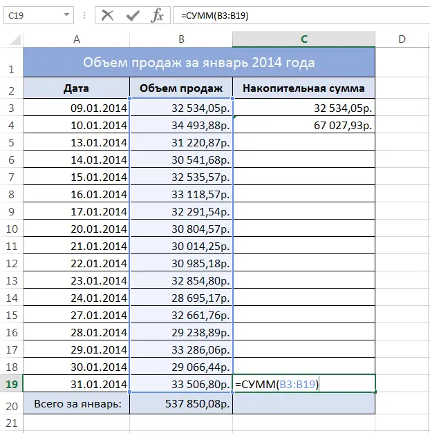
Cell C19 this formula: =SUM(B3:B19)
From the above formulas, it becomes obvious that the formula we need should use a mixed reference and look like this:
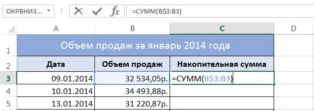
If we copy this formula to all cells of the table, we get the following result:
Since the values in cells B20 and C19 are the same, you can be sure that the cumulative sum in Excel is calculated correctly. As you can see, everything is simple!