


Contents
Have you ever wanted to plot two different (albeit related) datasets on the same chart? Perhaps you wanted to see the number of leads that came from several channels at the same time, and the conversion rate of these channels. Putting these two datasets on the same chart would be very helpful in discovering patterns and identifying trends that populate the funnel.
Lead (lead, target lead) – a potential client who in one way or another reacted to marketing communication. term lead it has become customary to designate a potential buyer, contact with him, received for subsequent managerial work with a client.
But there’s a problem. These two datasets have completely different dimensions. Y axes (number of leads and conversion rate) – as a result, the graph is very doubtful.
Fortunately, there is a simple solution. You need what is called secondary axle: with its help, you can use one common X-axis and two Y-axes of different dimensions. To help you with this annoying task, we’ll show you how to add a secondary axis to a chart in Excel on Mac and PC, as well as in Google Doc Spreadsheets.
How to Add a Secondary Axis to an Excel Chart on Mac
Step 1: Enter data into the table
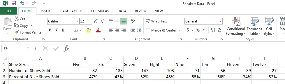
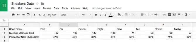
Let line 1 contain labels for the x-axis, and lines 2 and 3 contain labels for the two y-axes.

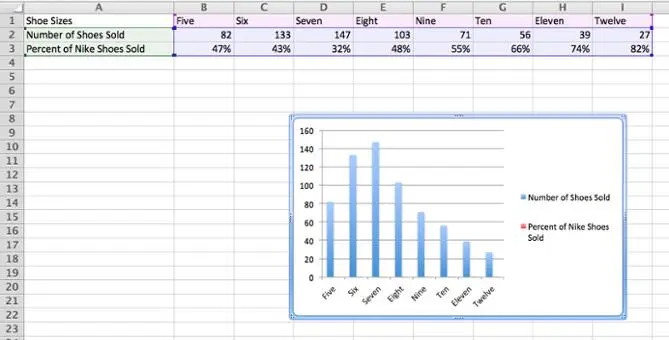
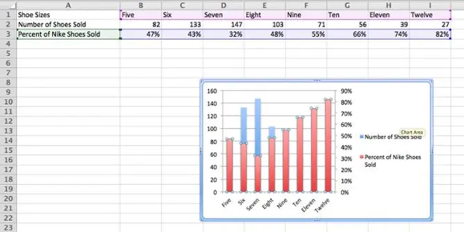
In this example, the first line shows the shoe sizes, the second line shows the number of shoes sold, and the third line shows the percentage of shoes sold.
Step 2: Create a chart from existing data
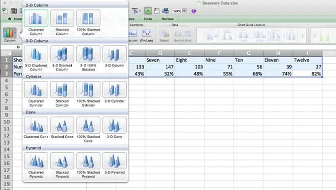
Select the data you want to show on the chart. Then click on the menu Diagrams (Charts), select bar chart (Column) and click the option Histogram with grouping (Clustered Column) top left.
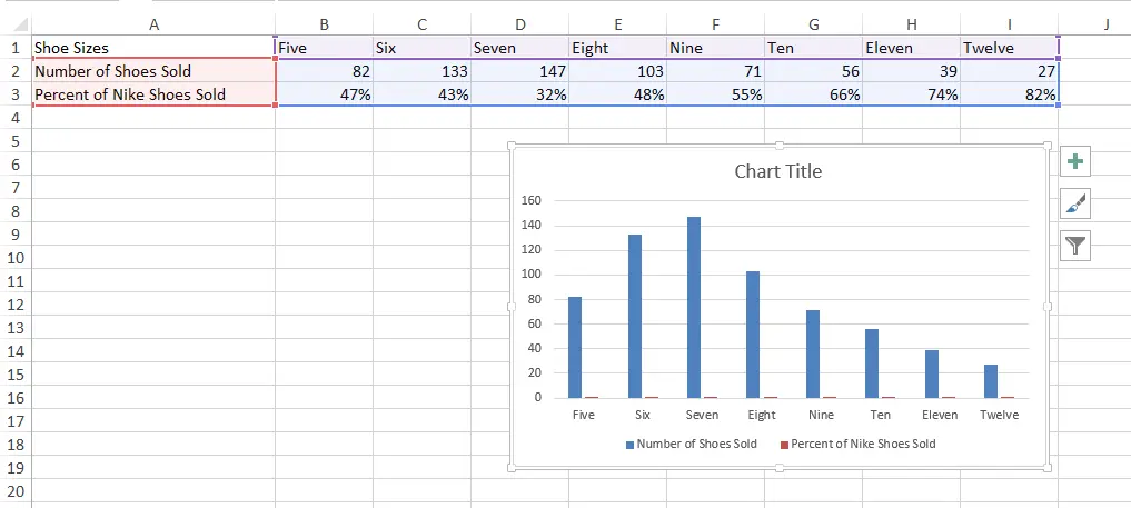
The chart will appear just below the data set.
Step 3: Adding a Secondary Axis
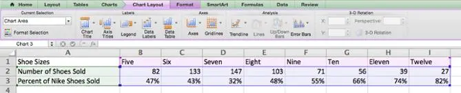
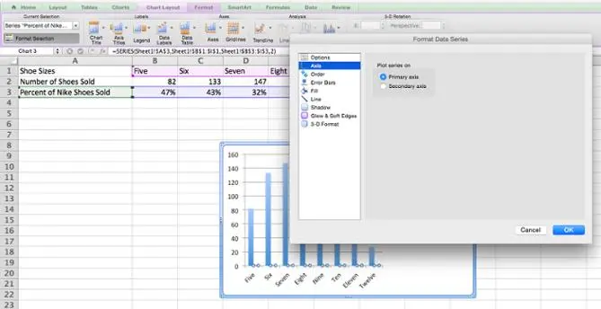
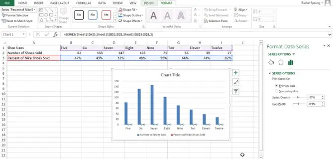
Now let’s build a graph along the auxiliary axis for the data from the row Percent of Nike Shoes Sold. Select the chart next to the menu Diagrams (Charts) a purple label should appear – chart layout (Chart Layout). We click on it.
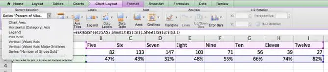
In the upper left corner in the section current fragment (Current selection) open the drop-down list and select Percent of Nike Shoes Sold or any other data series that needs to be plotted along the secondary axis.
When the desired data series is selected, press the button Selection Format (Format Selection) just below the dropdown list. A dialog box will appear in which you can select a secondary axis for plotting. If section Axes (Axis) did not open automatically, click on it in the menu on the left and select the option Secondary axle (Secondary Axis). After that click OK.
Step 4: Set up the formatting
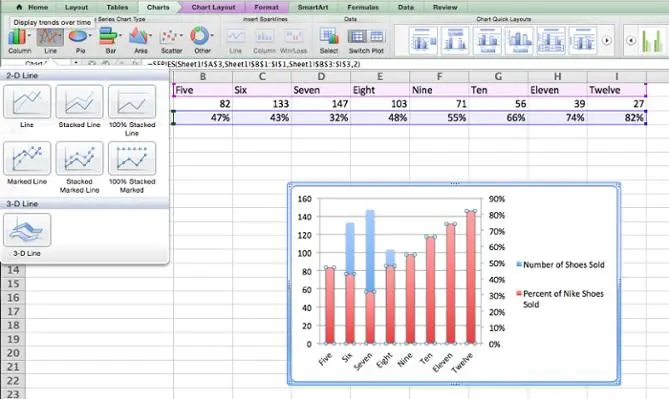
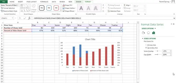
Now chart Percent of Nike Shoes Sold overlaps the graph Number of Shoes Sold. Let’s fix this.
Select the chart and click the green tab again Diagrams (Charts). Click on the top left Timetable > Timetable (Line > Line).
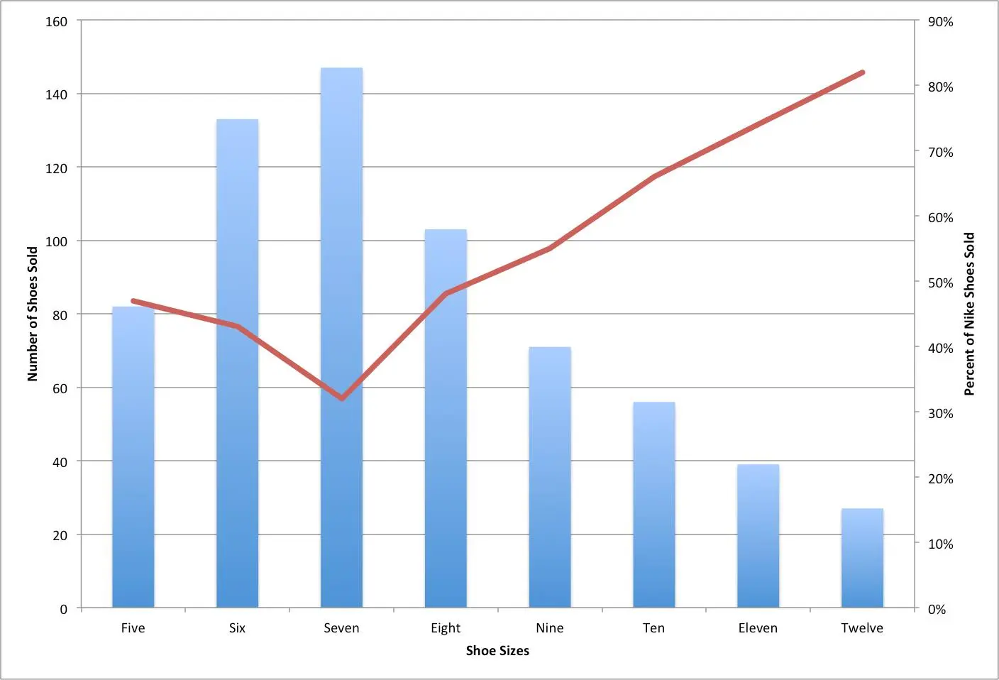
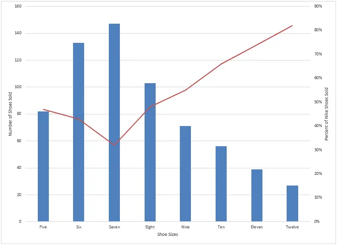
Voila! We have a chart that clearly shows the number of pairs of shoes sold and the percentage according to their sizes.
How to Add a Secondary Axis to an Excel Chart on Windows
Step 1: Add Data to the Sheet
Let line 1 contain labels for the x-axis, and lines 2 and 3 contain labels for the two y-axes.
Step 2: Create a chart from existing data
Select the data you want to show on the chart. Then open the tab Insert (Insert) and find the section Diagrams (Charts). Click on the small icon with vertical lines. A dialog box will open with several plotting options to choose from. Let’s choose the first one: Histogram with grouping (Clustered Column).
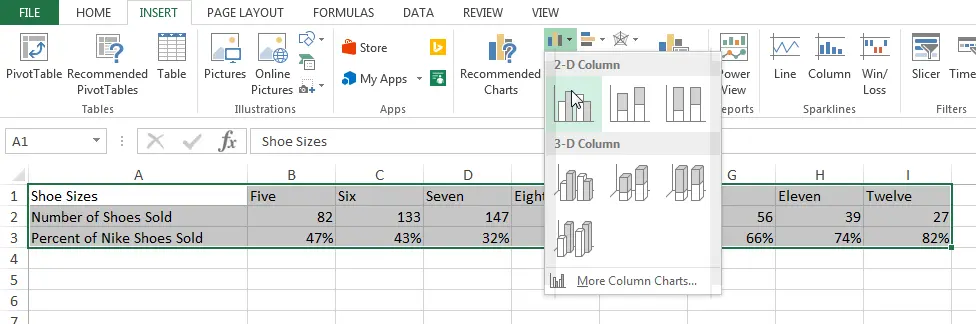
After clicking on this icon just below our data, a chart immediately appears.
Step 3: Adding a Secondary Axis
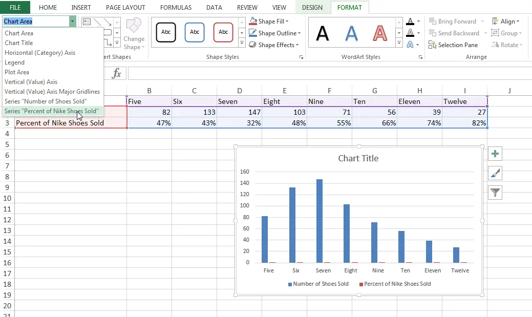
Now let’s display the data Percent of Nike Shoes Sold along the minor axis. After the chart was created, two additional tabs appeared on the Ribbon: Constructor (Design) Framework (Format). Opening a tab Framework (Format). On the left side of the tab in the section current fragment (Current Selection) expand the dropdown list Construction area (Chart Area). Select a row with a name Percent of Nike Shoes Sold – or any other series that should be built along the auxiliary axis. Then we press the button Selection Format (Format Selection), which is located immediately below the drop-down list.
In the right part of the window, the Format panel will appear with the section open Row Options (Series Options). Check the box Minor Axis (Secondary Axis).
Step 4: Set up the formatting
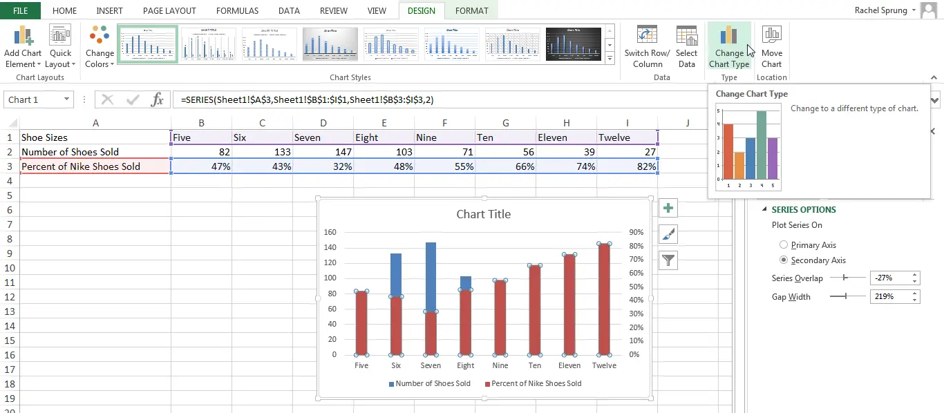
Note that the plot of the data series Percent of Nike Shoes Sold now overlaps the row Number of Shoes Sold. Let’s fix this.
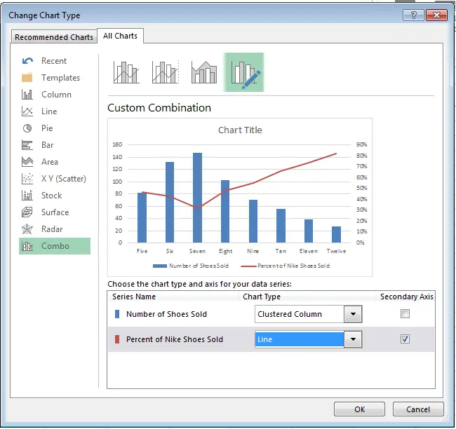
Click the Constructor (Design) and press Change chart type (Change Chart Type).
A dialog box will appear. At the bottom of the window next to Percent of Nike Shoes Sold click the drop down list and select build option Timetable (Line).
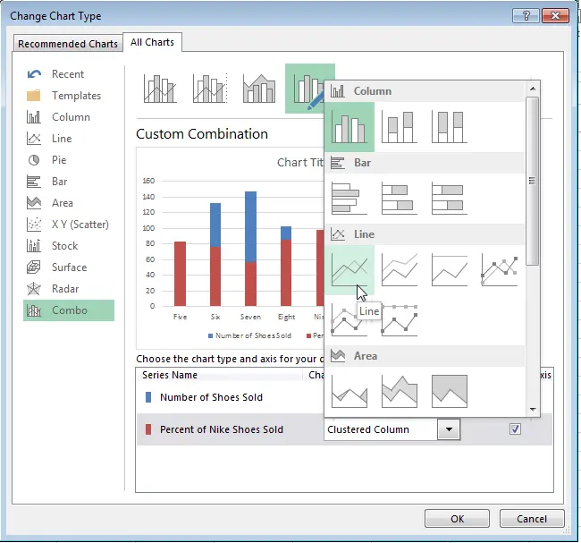
Make sure there is a checkmark next to this dropdown Secondary axle (Secondary Axis).
Voila! The chart is built!
How to Add a Secondary Axis in Google Doc Spreadsheets
Step 1: Add Data to the Sheet
Let line 1 contain labels for the x-axis, and lines 2 and 3 contain labels for the two y-axes.
Step 2: Create a chart from existing data
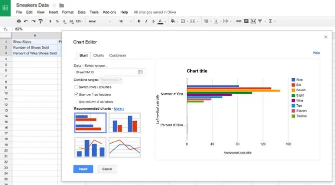
Highlight the data. Then go to the menu section Insert (Insert) and in the list that opens, click Diagram (Chart) – this item is closer to the end of the list. The following dialog box will appear:
Step 3: Adding a Secondary Axis
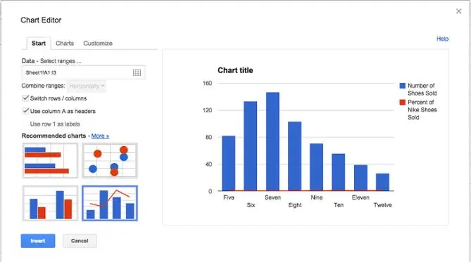
On the Advanced tab Recommended (Start) select a combo chart showing a bar chart with a line chart overlaid on it. If this option is not on the home screen, then by clicking the link Additionally (More) next to the title Recommended (Recommended charts) select it from the full list of options.
Parameter Headers – Column A Values (Use column A as headers) must be checked. If the chart looks wrong, try changing the setting Rows / columns (Switch rows / columns).
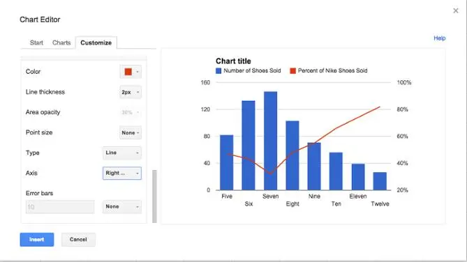
Step 4: Set up the formatting
It’s time to clean up the formatting. On the tab Setting (Customize) scroll down to the section series (Series). Expand the drop-down list and select the name of the auxiliary axis, in our case it is Percent of Nike Shoes Sold. In drop down list Axis (Axis) changes Left axis (Left) on Right axis (Right). Now the minor axis will be clearly visible on the chart. Next, press the button Insert (Insert) to place the chart on the sheet.
Voila! The diagram is ready.
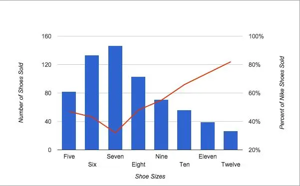
And what data are you plotting along the auxiliary axis?