


Contents
In the previous article, we talked about how to create a spreadsheet in Excel and explored several ways to make it really interesting. In the second part of the article, we will dig even deeper and analyze several new features of tables. You will learn how you can make a table and a project as a whole really stand out!
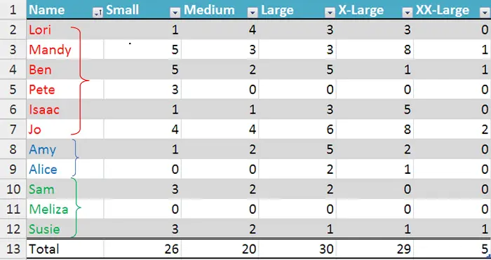
So, in the table below, we see the receipts from the sale of T-shirts by a certain group of people. The first column contains the names of the members of the group, and the rest – who sold how many T-shirts and what size. Now that we have a table to work with, let’s take a look at the various things we can do that we couldn’t do with a simple range of data in Excel.
Total Rows in an Excel Table
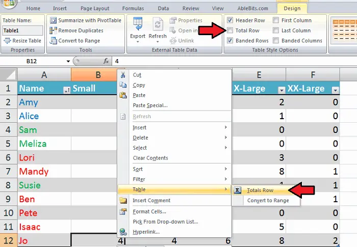
The figure above shows what our data table looks like. First you need to sum up for each size of T-shirts. If I wanted to do this while working with a range of data (not creating a table), I would have to manually enter formulas into the cells where the totals would be located. With a table, everything is much easier! All I have to do is enable the corresponding option in the menu and the total row will automatically appear in the table. Right-click anywhere in the table, in the context menu select Table (Table) and beyond Total Row (Total row). Or just check the box next to the option Total Row (Total row) on the tab Design (Constructor) section Table Style Options (Table style options).
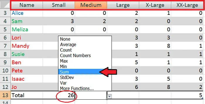
Now at the bottom of the table there is a row with totals. Expand the drop-down menu – here you can select one of the mathematical functions: Average (Average), Count (Quantity), Max (Maximum), StdDev (Offset deviation) and many other functions if you press More Functions (Other features). The function range is selected automatically. I chose Sum (Amount), because want to know the amount of T-shirts sold for this column (or you can use the keys Ctrl + Shift + T).
Tip: Did you pay attention to the top line? This is another advantage of tables! If the data is stored as a simple range, you will need to freeze the top row to always see the headers. When you convert the data to a table, the column headings are automatically fixed at the top when you scroll down the table. It’s very user friendly!
Automatic insertion of formulas in all cells of a column
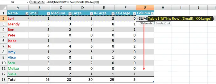
You may not know it, but Excel is always trying to anticipate what your next step will be. I added a column at the end of the table to summarize the sales for each person. By pasting the formula in the first row, it was automatically copied to the rest of the cells so that the entire column is now filled with totals! If you decide to add another row, the formula will appear in it too, i.e. data will always be up to date!
Sorting
I love using the context menu (right click). If there are some little extra steps in Microsoft apps that can be done, you will definitely find them there! Now I’ll show you how to get the most out of right-clicking when working with tables.
I need to see which sellers have already paid the prepayment for the T-shirts sold in order to prepare their orders. To do this, let’s sort by the first column. I changed the text in the table so that you can see who paid (green), who did not pay (red) and whose documents are missing (blue). I want to organize this information and I can do it. Of course, you can move each row manually… or Excel can do it for you!
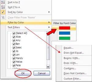
Click the dropdown menu next to the column heading Name, hover over the item Sort by Color (Sort by Color) and select the red font color.
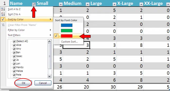
Below is what our table looks like. All red, blue and green colors are grouped together. Now I know who to shake about the payment!
Filtration
But our possibilities for working with data are not limited to this! You can organize information in many other different ways, including the ability to show and hide certain information. If I need to see people in red, I can filter by that color (note that you can just as easily filter by different text values, characters, and so on).
A wonderful property of tables: Depending on what manipulations you perform in the table, the totals always correspond to the data that is currently visible.
Allocation
Now let’s see how easy it is to make changes to the table.
Highlighting in tables is very easy. When we want to select a specific row or column in a range, we need to drag the mouse over the entire row or column, and this can be quite tedious, especially if the amount of data is very large. But only not working with tables!
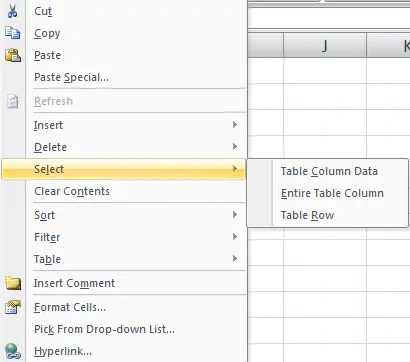
If you select one or more table cells, then right-click and hover over Select (Select), you will be given three options to choose from: Table Column Data (data in table column), Entire Table Column (Entire table column) or TableRow (Table row).
Again, this can be especially useful when there is a large spreadsheet on the Excel sheet.
Removal
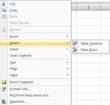
If you need to get rid of an unnecessary row or column, we follow the same steps, only this time select from the menu Delete (Delete). We will be prompted to delete either a column or a row. Note that the selected cell will also be deleted.
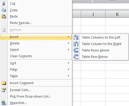
Insert
Do you need to add a column or row? Right-click again and in the context menu we find the item Insertion (Insert), and then select the option that we need. Another quick way to insert a new row is to select the last cell in the last row of the table (before the total row) and press Tab.
Tip: Have you noticed that the formulas in the total row and the formatting have been updated? If you have a chart, it will also be updated. If everything is done in a table, then there is no need to change the formulas or update the data for the chart, as you would with a normal data range.
If you’re using a complex formula, you can always use column names instead of A, B, C, and so on… this is another nice feature of tables that makes working in Excel much easier.
Sort, filter, table
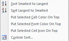
There are a few more actions that you can do using the context menu. We have previously talked about accessing the dropdown menu in a column header. Well, all this can be done with a right-click. You can sort by color, font, from largest to smallest or vice versa, and if there is no suitable sorting type, you can always set up your own.
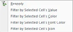
In addition, you can set up a filter in the context menu. Filter by color, font, icon, value – everything that you do not want to see will be hidden, and only what you need will remain.
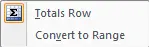
Remember we talked about summarizing with a tab Design (Constructor) – all this is easy to do using the right mouse button. Here you can create a total row (the data range will be selected automatically) or convert the table back to a range. All formatting and data will be saved, and if you are a master of hotkeys, you can press Ctrl + Shift + T.
Tip: If you want to learn more hotkey combinations, just hover your mouse over the menu item of interest. If there is a hotkey, the corresponding tooltip will appear!
Table Tools / Design tab
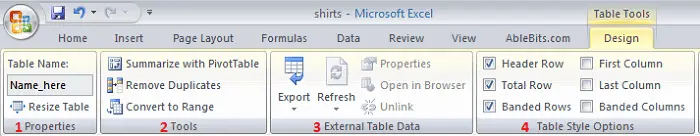
You didn’t think of that, did you? Yes… you can do a lot more interesting things with tables!!! Let’s see what groups of commands the tab consists of Design (Constructor):
- Properties (Properties). By giving the table a name, we can use that name when creating formulas and links. If you want to resize the table, use the command Resize Table (table size). You can select a new area of the table by dragging the mouse, or enter the coordinates of this area in a special field using the keyboard (for more details, see the first part of the article on tables).
- tools (Service). Team Summarize with PivotTable (Pivot table) makes it possible to present information in a modified form. If you are unfamiliar with this function, it might be a bit confusing at first, but it is another useful tool that you would not be able to use with a normal range of data. Using the command Remove Duplicates (Remove Duplicates) You will be able to remove duplicates quickly and without the hassle of searching through the entire table. Or you can convert the table back to a regular range by clicking the button Convert to Range (Convert to Range) – remember, in this case, all data will remain the same, but you will not be able to use the luxurious features of tables.
- External Table Data (Data from external table). This group contains commands that are needed to use the table outside of Excel. Here you can export the table to external resources such as SharePoint or Visio. If you did this, then changed something in your table and now you want to update the information on an external resource, just click the command refresh (Update). In this section, you can also check the properties of the data range, open the server version of the table in a browser, or disconnect from the server.
Tip: Remember that the last four tools are only available after you have exported your spreadsheet to an external resource. Otherwise, these functions cannot be used.
- Table Style Options (Table style options). Basically, these are formatting tools, and very useful ones! Remember we talked about the title bar that always remains visible while scrolling through the table (as an alternative to pinning the pane)? Here you can choose whether to display this header row at the top of the table. To do this, you need to check or uncheck the corresponding checkbox. In addition, we studied the totals line, which can also be enabled in this menu and achieve the same result. Finally, options Banded Rows (interleaved lines), Banded Columns (Striped columns), First Column (First column) and Last Column (Last column). Each of these options adds color highlighting to the respective rows or columns to highlight the information you need. I like to use these options because they help me find the part of the table that I want to focus on.
All of these tools are designed to help create the most functional table. Perhaps we do not always use them, but if you at least know that such an opportunity exists, then in the future it will definitely come in handy and give a serious advantage.
Data formatting may seem like the most important task, but it doesn’t have to be. Letting Excel do the work for you in a spreadsheet format will take you one step closer to making your life much easier. The first part taught us how to create a spreadsheet in Excel, and the second part showed us how to get down to business in order to get the most out of what Microsoft has to offer for creating spreadsheets.
Work with tables – it’s as easy as just entering data. Study the context menu, try everything you find in it. Whether it’s inserting or deleting… sorting or filtering… or even just formatting, you’ll find that working with tables is much easier and more convenient than working with ranges of data.
Enjoy it!