Contents
Formulation of the problem
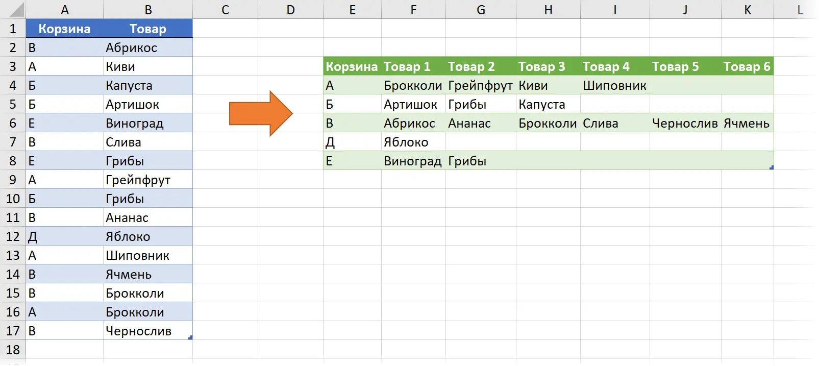
We have a list of objects (for example, goods) with a mark to which set (basket) each of them belongs. It is necessary to decompose the objects into their sets, forming a table as in the figure on the right:
Similar tasks are encountered in practice quite often – in cases where it is necessary to allocate certain resources:
- team members
- drivers on routes
- clients by managers
- goods in baskets, etc.
In the past, I already made an article and video about a similar task, where we figured out how to shift a one-dimensional column with data into a two-dimensional table, but the situation was simpler there, because each set (row) had the same size (number of columns). Here, the number of elements in the sets is not known in advance and is not equal to each other, so the approach will have to be changed.
So that you have a choice, let’s look at several ways to solve this problem.
Method 1. Manually through a pivot table
This method does not involve automatic updates, so it is only suitable in cases where you need to simply, quickly and one-time solve such a problem. We do the following:
1. We put the active cell in any place of the source table and build a summary cell on it through Insert – PivotTable (Insert — Pivot Table).
2. In the fields panel of the summary we drop the field Bin to the area of lines, field Product — to the area of columns and to the area of values. At the output, you should get a summary, where at the intersection of the basket and the product there will be a number if the product is included in the specified basket:

3. We select the central data area in the summary, not including the totals (range E3: S8 in the example above), copy and paste with a special paste as values into any place on the sheet.
4. In the copied range, select again only the central block with numbers without labels and then force Excel to select only the cells with numbers by pressing the key F5 – button Highlight — Constants (F5 — Go to Special — Constants):
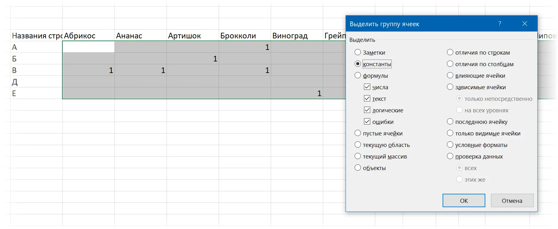
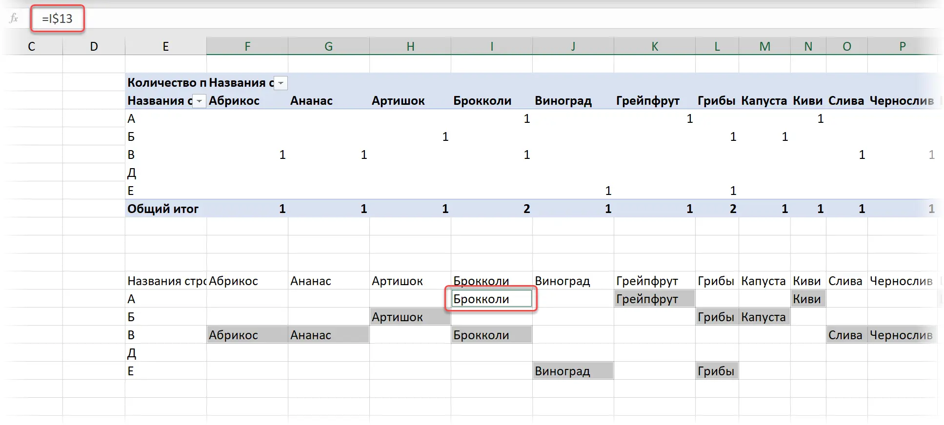
5. Carefully, so as not to knock down the resulting selection, enter in the first selected cell (it will be white) a link to the product corresponding to it (in our case it will be a link to Broccoli), press the key F4to leave the dollar sign in front of the number only (i.e. freeze the string) and keyboard shortcut Ctrl+Enter (to enter similar formulas in all selected cells at once):
6. We replace formulas with values in the entire table with a special insert.
7. Using the trick with the key already familiar from paragraph 4 F5 — Highlight this time, select the empty cells and delete them with a shift to the left:
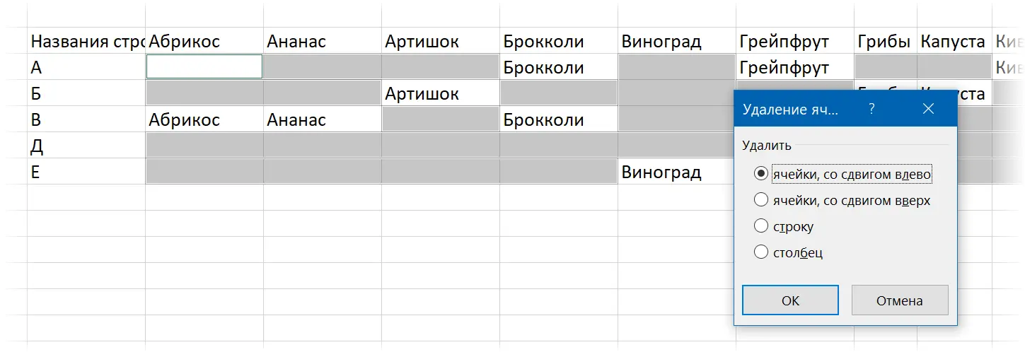
The problem is solved.
Method 2: Updatable query via Power Query
This method is a little more complicated, but it will allow us not to repeat the whole process in the future when the initial data changes – it will be enough just to update our query. We will use the Power Query add-in for the solution, which for Excel 2010-2013 can be downloaded for free from the Microsoft website. Starting with Excel 2016, Power Query is already built into Microsoft Excel by default.
To solve our problem, we do the following:
1. We turn the original table into a dynamic “smart” table so as not to think about changing its size later. You can use the command Home – Format as a table (Home — Format as Table) or keyboard shortcut Ctrl+T.
2. We load the resulting “smart” table into Power Query through the command Data – From Table/Range (Data — From Table/Range).
3. If we want the goods in each basket to be in alphabetical order, we sort the table first by baskets, and then by goods, using the filter buttons in the table header.
4. We group the table by baskets by selecting on the tab Transformation Command Group by (Transform — Group by) and setting as operation All lines (All rows):
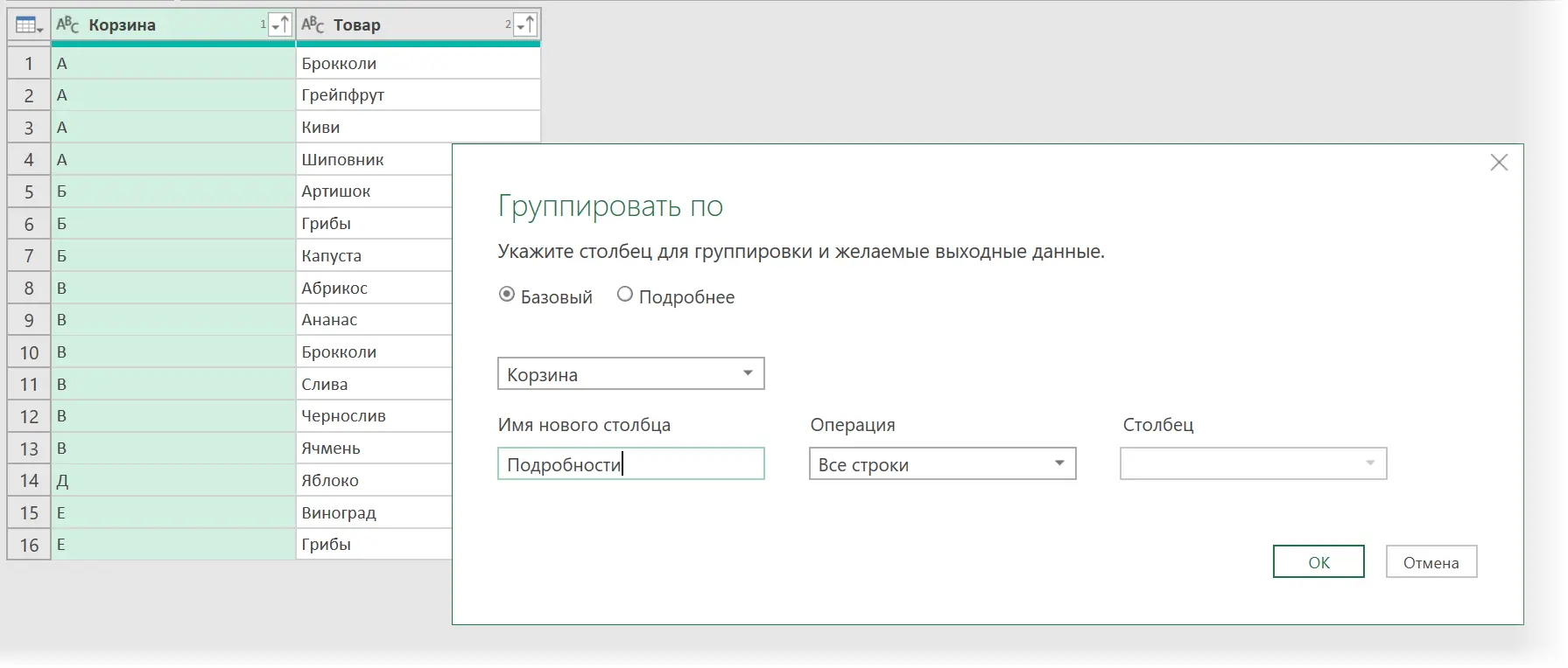
Our original table will “collapse” to the baskets, the contents of which will lie in nested tables in the last column:
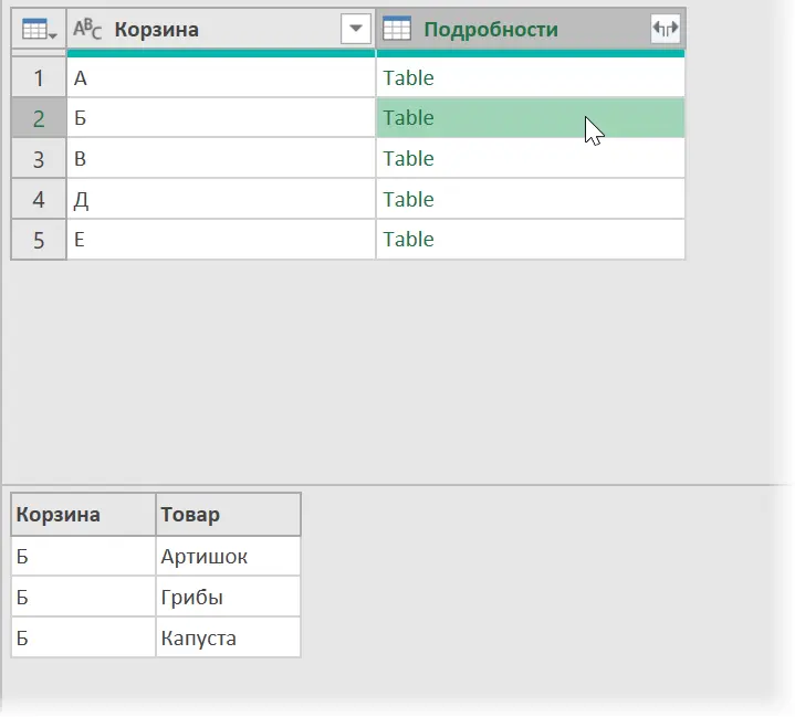
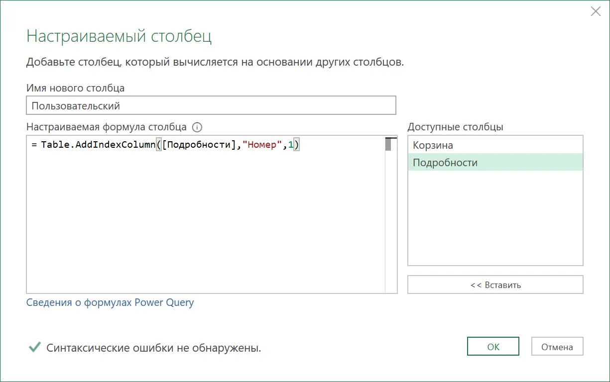
5. Choose a team Adding a Column – Custom Column (Add Column — Custom column)to add an index column to each nested table with row ordinal number using the M-function Table.AddIndexColumn:
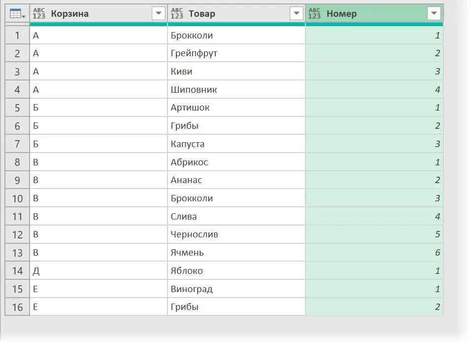
6. We delete all columns except the last one, and expand its contents with an icon with double arrows in the table header. We get, in fact, the original table, but with the added numbering of goods inside each basket:
7. We add the word “Product” in the last column to the numbering using the command Transform – Format – Add Prefix (Transform — Format — Add Prefix).
8. Finishing touch: we perform a collapse on the last column with numbering using the command Transform – Pivot Column (Transform — Pivot Column):
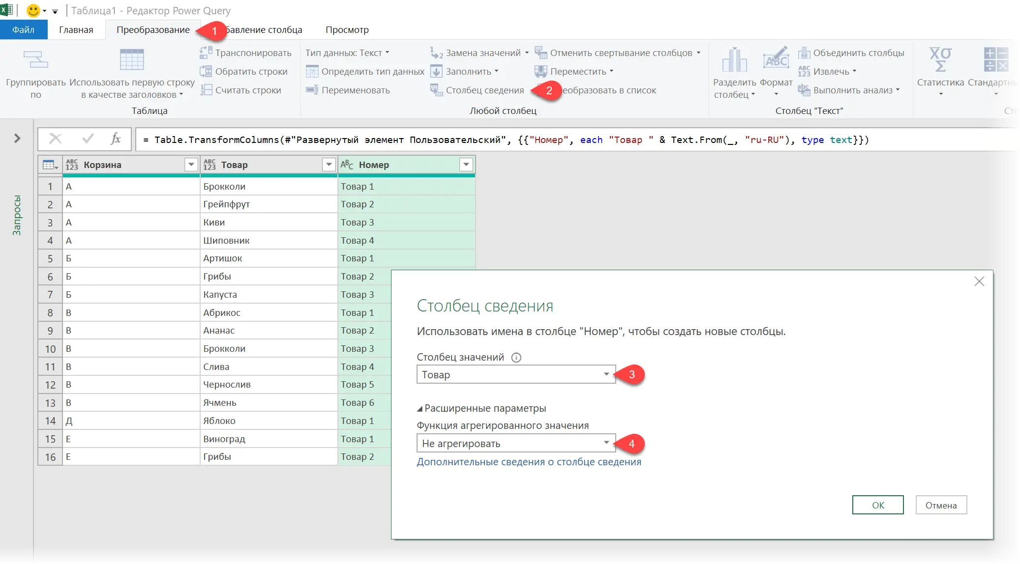
Problem solved! It remains to upload the results back to Excel via Home — Close and Load — Close and Load in… (Home — Close & Load — Close & Load to…)
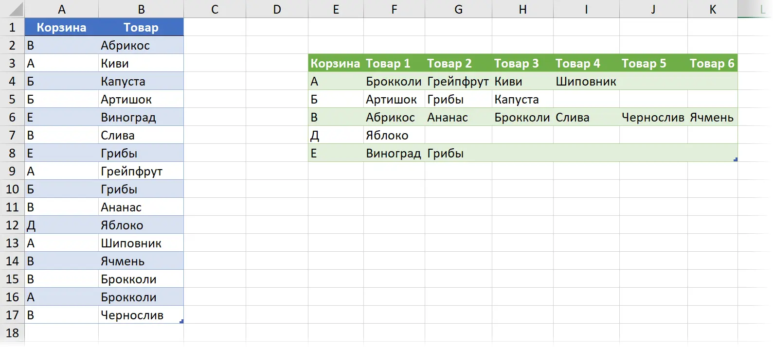
When changing data in the source table, we will need to update our query by right-clicking on the resulting table and selecting the command Update & Save (Refresh) or button Update All tab Data (Data — Refresh All).
Method 3. Dynamic array functions
This method is only suitable for those who have the latest Office 365 updates installed, which added support for dynamic arrays to Excel functionality and new functions for working with them: SORT, UNIQUE, FILTER, LAST and RANDOM. If you have Office 365, but don’t have these features yet, then the corresponding updates have not yet reached you (they are sent in waves and not to all users at once), so you need to wait a bit.
This method is good, first of all, because with any changes in the source data, the results are updated “on the fly” automatically. And the process itself is not very complicated – you only need three formulas.
Let’s go:
1. We turn the original table into a dynamic “smart” table so as not to think about changing its size later. You can use the command Home – Format as a table (Home — Format as Table) or keyboard shortcut Ctrl+T.
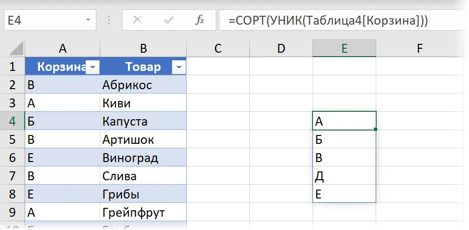
2. Forming a sorted list of unique cart names from a column [Basket] our smart table Table 4 – using functions GRADE (SORT) и UNIK (UNIQUE), respectively:
3. We display all products from each basket using the function FILTER (FILTER):
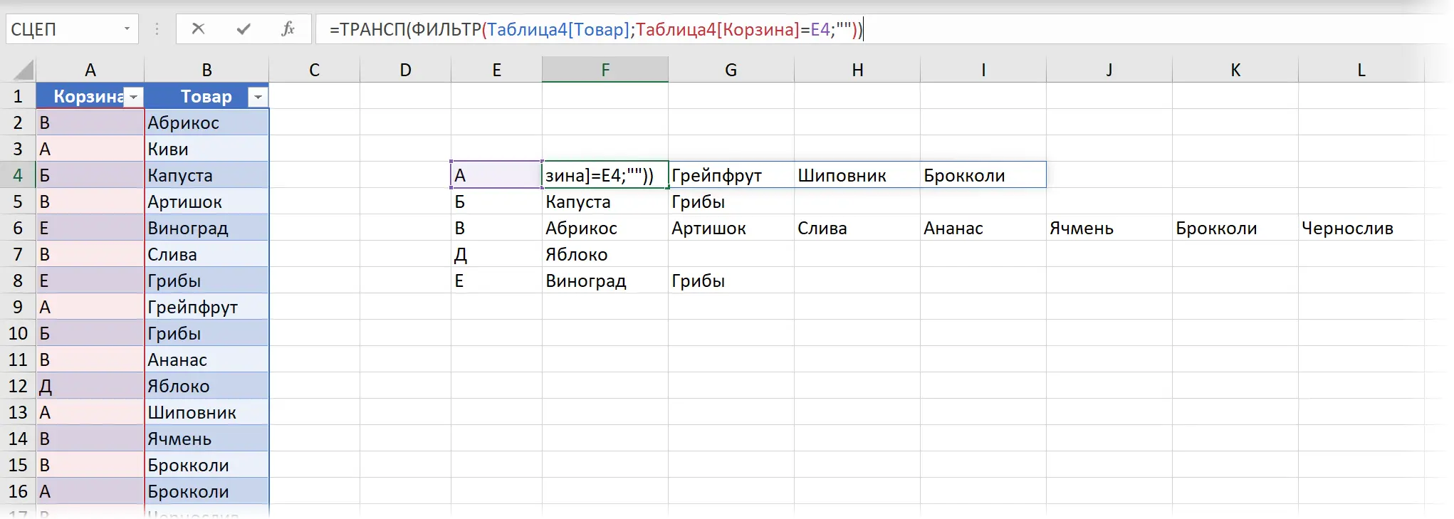
By default, the function FILTER prints the results in a column. To expand them horizontally – into a line – we additionally use the transposition function TRANSP (TRANSPOSE).
4. Add a hat for beauty:

Here the logic is:
- Function COUNTIF (COUNTIF) calculates an array with the size of each basket – this, in our case, will be {4,2,7,1,2}
- Then the function MAX (MAX) determines the largest number in it (7)
- New Dynamic Arrays Feature AFTERBIRTH (SEQUENCE) generates a numerical sequence from 1 to 7, to which the word “Product” is then glued to the beginning.
- Dynamic arrays are a silent revolution in Excel
- Transforming a column into a table (using formulas and using Power Query)
- Turning rows into columns and vice versa


