Creating a Pie Chart in Excel

This article has complete instructions for creating charts, adding and removing legends, formatting, and other aspects.

First you need to define what a pie chart is. This is an element that allows you to display the ratio of the part to the whole. Its value is always 100%, and the percentage of the sectors themselves can be specified independently.

Regular users enjoy working with pie charts because they display data in a simple and understandable way. However, some experts consider their use unnecessary. The main reason for this is the fact that people often create sectors on their own “by eye” whose size does not correspond to the percentage presented.

Not using pie charts at all is at least unreasonable. That is why you should learn how to create them correctly. If you’re charting by hand, there’s a good chance the highlighted part won’t match the actual percentage.

Fortunately, Excel provides additional options for creating charts with live data. They can be formatted and set size, color, etc.

The process of creating a chart

Adding this element to the sheet takes a little time. Particular attention should be paid to the order of indicators and the type of future chart.

1. Prepare the data

The main feature of the chart is the fact that it can be made on the basis of indicators from one column or row. That is why it contains only one row of data.

When copying the required indicators, you can also highlight the category names. After that, they will be displayed in the legend and captions. A chart is well done if:

It has only 1 row with values.
The numbers are greater than or equal to zero.
There are no empty sectors.
There are not too many segments.

Here the chart is created based on the following metrics: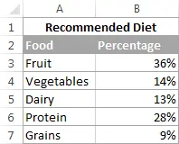

2. Add a chart

Select the required indicators and go to the section “Insert”. There you will need to specify the type of future diagram. We decided to create a two-dimensional chart: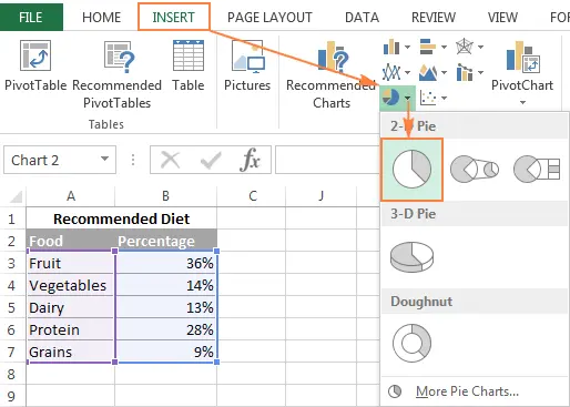

Note: to have the name of a column or row also used as a heading, simply highlight it along with the data.

3. Format your chart

Once created, go to “Designer”, find the option “Diagrams” and apply any style you like.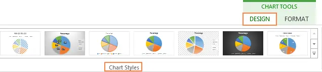

There is no denying that the diagram looks simple enough.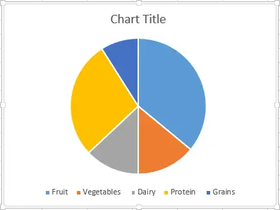

To make its appearance more understandable and data display simple, it is worth adding a title and captions and changing the color scheme. We will talk about these aspects soon, but first it is advisable to consider the types of charts.

Basic principles of working with different charts

The program presents a variety of charts, use any of them.

2D Diagrams

Perhaps most often in Excel they work with a 2D chart. It can be done simply and quickly. Switch to “Insert”, find the section “Diagrams” and add it.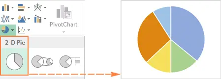

3D Diagrams

This type is similar to the previous ones. However, on such charts there is additional data located on the depth axis.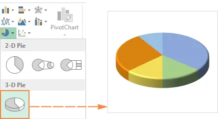

If you choose this particular type, you can use additional options.

Secondary charts

If you are making a complex chart with many sectors, which in turn are subdivided into small parts, then this type is what you need.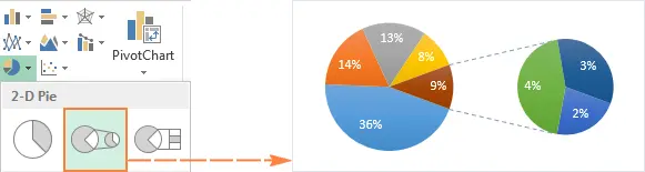

Additional data will appear on the second smaller element, as shown in the screenshot below.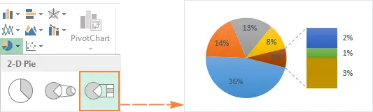

When creating such diagrams, the last 3 categories with indicators will be displayed on an additional graph. To avoid problems, do the following:

arrange the indicators in descending order so that the lowest values are moved to the new chart;
independently select the indicators that you want to move to the second chart.

Create categories for an additional chart

If you want to select the data that will be displayed on the secondary chart, then follow this instruction:

Click on the sector and find “Data Series Format”;
В “Row Options” indicate “Split Row” and adjust the necessary parameters:
- Position – will help to determine the categories that need to be transferred to an additional diagram.
- Value – allows you to specify the value threshold at which data will be displayed in the secondary chart.
- Percent – similar to the “Value” parameter, but in this case you must specify a percentage.
- Other – this option will allow you to choose the sectors that will be transferred.

Most often, the best option is to choose the option “Percentage”. You can see the use of this parameter in the screenshot below: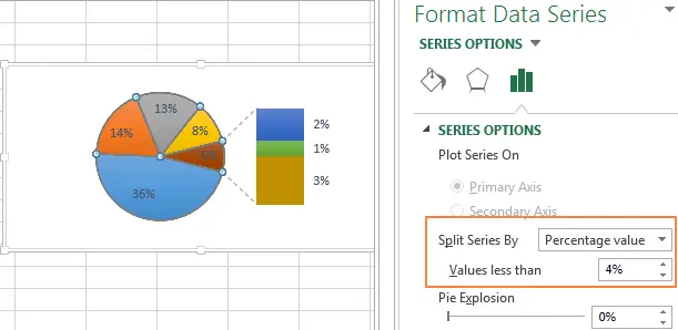

It should be noted that you can make changes to additional options:

Side clearance – measured as a percentage, the parameter determines the distance between the primary and secondary diagrams. To adjust it, move the slider or enter a number in the special field.
Secondary Chart Size… Please select “Size of the second construction area” and adjust the setting using the slider or enter a number in the field.

Donut charts

When you work with large amounts of information, it makes sense to use a donut chart. However, it should be noted that the indicators in it are not displayed so clearly and clearly. Instead, we would advise using a histogram: all the data is placed on it more logically, making their perception easier.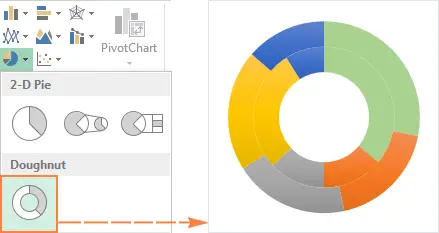

Inner Ring Size Adjustment

When working with this type of chart, not only sectors are visible, but also an empty hole in the middle. To adjust its size, follow a few simple steps:

Click on the sector and click on the option “Data Series Format”;
Switch to “Row Options” and adjust the diameter of the inner circle by moving the slider or entering a certain number in the box.

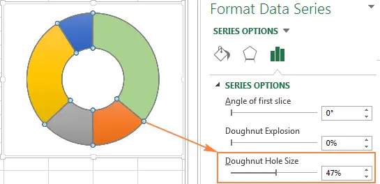
Chart customization

If you only need to control the data and determine the trends in its change, then the knowledge gained will be enough for you. However, if you need to create visual diagrams that other people will analyze, then you will need additional knowledge to improve their appearance. You can read about customizing and formatting these elements below.

How to make chart captions

By labeling data, you can more easily understand and analyze the information presented. The program has the ability to add labels both to all data and to some fragments.

Creating signatures

Here we will add labels to all chart data. To do this, click on the icon with a green cross and find “Data Signatures”.

Note that the position of the labels can be adjusted by clicking on the special arrow, which is located to the right of the parameter. Excel provides a variety of options for displaying data.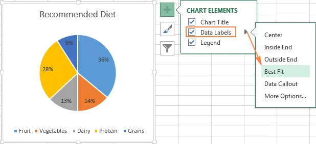

So, you can move labels outside the diagram. To do this, simply select the option “Data Callout”: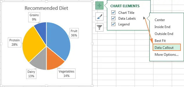

If all the inscriptions are placed inside the sectors, then, most likely, some of them will be almost impossible to read. Initially, the text color is black, which is why it is barely noticeable on fragments with a dark background. To change the color of the text, go to the tab “Format” and select the option “Color Fill”. You can also select a different sector fill here.

Show categories in labels

If there are more than three sectors on the diagram, then the name of the categories can be written directly on them. When working, you will not need to go to the legend to find out which indicator is displayed. This will save you time and improve the perception of information.

To apply this option, go to the tab “Constructor”, then find “Chart Layouts” and specify “Express Styles”. You can see that on the first and fourth layouts, the inscriptions are on the sectors themselves: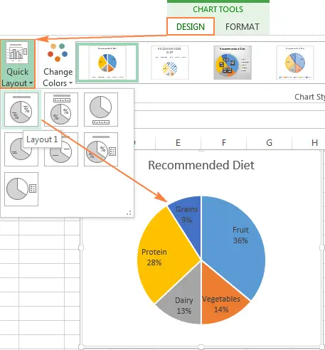

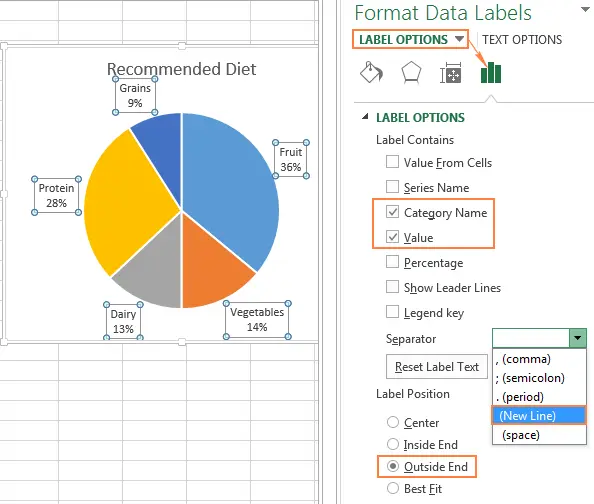
To configure additional settings, click on the icon with a green cross, then on the arrow and select the option “Extra options”. In the panel that opens, go to the tab “Signature Options” and click on the field “Category Name”.

You may also need additional options:

Parameter “Include in Signature” will allow you to select the indicators that will be displayed in the signature;
On the menu “Separator” you can find the necessary way to separate indicators;
Using option “Label Position” you can set the location of the signature.

Note: when the chart itself has labels, you can get rid of the legend. Remove it by clicking on “Chart elements” and removing the checkbox next to the title “Legend”.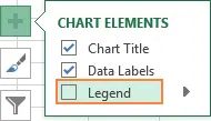

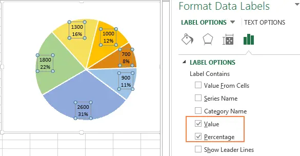
Percent display

If you have chosen to display indicators as a percentage, they will appear on the signatures after enabling the option “Data Signatures” tab “Chart elements” or choice “Meaning” on the panel “Data Signature Format”. This is shown in the previous screenshots.

If the indicators are indicated in numbers, then you can configure their display without changing or replace them with percentages. In addition, you can make both a numeric value and a percentage value be displayed at the same time.

Click on a segment and find the parameter “Data Label Format”.
Выберите “Meaning” or “Percentage”.

Dividing the chart into sectors or selecting one fragment

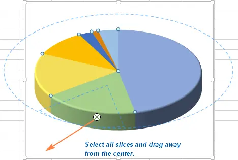
To more visually present individual indicators, divide the chart into fragments. Thus, the sectors will not touch each other and will be further from the center. In addition, to emphasize only one fragment, you can move only it.

It should be noted that any chart can be split: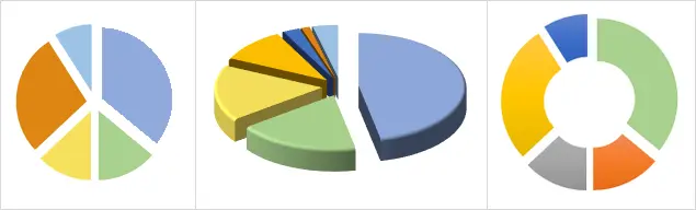

Break the whole diagram into fragments

The diagram can be divided into fragments as follows:

Click on an element and select all sectors.
Move them to the side with the mouse.

If you want to do everything accurately and evenly, then follow these instructions:

Highlight a sector and select “Data Series Format”.
Find a tab “Row Options” and move the slider to increase or decrease the gap. You can also just enter a number in the field:

Separate one piece of the chart

To draw attention to an important sector, it can be separated from the diagram. So he will stand out from others and will not go unnoticed.

The easiest way to do this is to select the required fragment and move it further away. To select only one part, double-click on it.

There is an additional effective way: select a sector, click on it and find “Data Series Format”. After that, you will need to go to “Row Options” and adjust option “Point Cut”.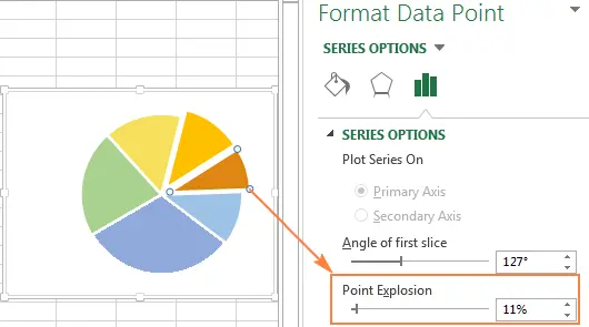

Note: if you need to separate more than one sector, then you will have to repeat the above steps with each segment. Unfortunately, it is impossible to select several fragments and move them at once.

Pie Rotation

The order of the categories depends entirely on the order in which the indicators are initially placed. However, you have the option to rotate it however you like. Elements that have small segments in front are best perceived.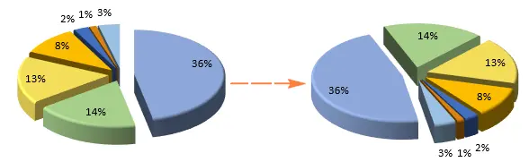

To expand a chart, follow these steps:

Click on a segment and find “Data Series Format»;
In section “Row Options” find an option “Angle of rotation of the first sector”.

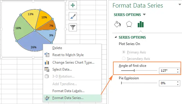
Move the slider and adjust the rotation angle. You can also just enter a numeric value in a special field.

Additional Options for Rotating 3D Charts

If you prefer to use XNUMXD charts, then you can set up additional options. To find them, click on any fragment and select “Rotation of a three-dimensional figure”.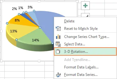

You will see a special panel “Chart Area Format”. There you can adjust additional settings:

Horizontal rotation;
Vertical rotation;
Viewing angle.

Note: charts can only be rotated around two axes: X and Y. The depth parameter does not affect the rotation of this element in any way.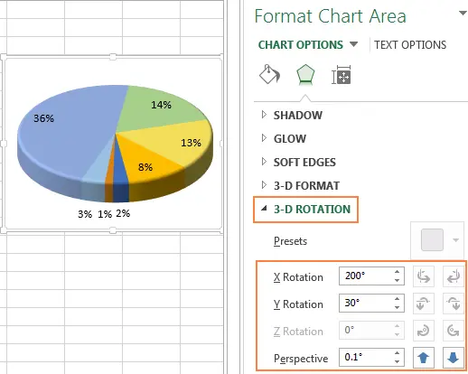

Click on the arrows next to the options to rotate the chart. Its position will change slightly, so you can achieve the ideal position.

Sorting segments by size

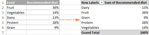
Statistical data is easier to understand when the sectors are placed next to each other in ascending order. To make this type of chart, you can sort the data on the sheet. However, if this is not possible, follow these instructions:

Make a pivot table that will present the necessary values;
Place the names in the field “Line”, and the numbers are in “Values”… It will look like this:
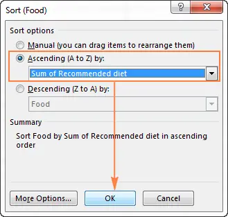
next to option “Line Names” click on the icon “Autofilter” and specify “More Sort Options”;
Choose the type of sorting that suits you:
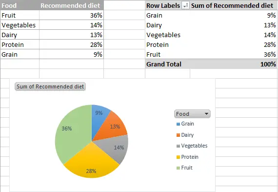
Create a chart based on this table.

Change chart color settings

If you don’t like the default color scheme, you can customize it yourself. There are several options:

Change the color scheme completely;
Change the fill of individual fragments.

Change the color of the entire chart

If you want to completely change the color scheme, click on the icon with a green cross, go to the “Color” and choose any theme you like.

You can simply click on the diagram to display an additional group at the top “Working with charts”. Switch to “Designer” and find the option “Chart Styles”. You will then need to click on “Change Colors”: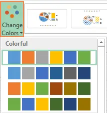

Changing the color of an individual sector

Of course, the number of color schemes is very limited. If you need to prepare a unique and memorable diagram, then choose a special shade for each segment.

To change the color of a fragment, double-click on it. On the tab “Format” find the parameter “shape fill”. After that, you can assign any color to the fragment.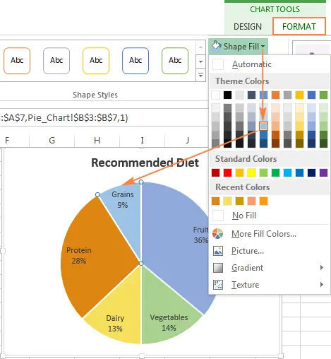

Note: small segments with insignificant indicators should be grayed out. So, they will not distract attention from the main data, and at the same time they will be displayed on the chart.

Chart Formatting

When creating a diagram, you can customize its appearance to make it even more understandable and memorable.

Click on the diagram and select an option “Data Series Format”. After that, you can adjust the shadow, glow, and anti-aliasing.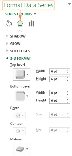

In section “Format” you will also find additional features:

Chart size adjustment;
Setting the color of the entire chart and its outline;
Application of additional effects;
Using styles to change text;
And others.

To use these options, select the fragment you want to edit. After that go to “Format”. Those functions that can be applied will be highlighted in normal color. Inactive options will be grayed out and cannot be selected.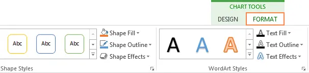

Pie Chart Notes

So, now you know everything about creating charts in Excel. Let’s summarize and define a list of important actions. In addition, you must specify what you definitely should not do:

Sort sectors in ascending order. To make the data easier to understand, arrange the fragments from largest to smallest.
Merge sectors. If there are too many sectors in the chart, then they should be grouped into large fragments. After that, assign a specific color to each group of data – this way the data will be easier to perceive.
Highlight small sectors with a soft color. If your chart has a lot of small segments, make them gray or put them in the “Other” group.
Expand the chart. Small fragments will be in front, which will make the presentation of data more understandable.
Do not add a lot of information – choose only the most basic indicators. If there are too many sectors on the chart, it will make it difficult to read. When working with more than 7 categories, consider creating a secondary pie (or bar) chart. Small categories can be moved to an additional element.
Remove the legend. Consider creating labels right on the chart so you don’t have to waste time jumping to the legend.
Refrain from using multiple 3D effects. Don’t use too many XNUMXD effects as they will make the diagram less attractive and distort the text.

That’s all. Soon we will talk about creating histograms and working with them. Stay tuned and learn more about useful options in Excel!