


Contents
Helen Bradley explains some of the PivotTable formatting differences in Excel 2010.
With the release of Excel 2007, Microsoft has added some additional conditional formatting features, such as bar charts and icon sets, which allow you to visualize the relative values in these cells.
Microsoft has made changes to how conditional formatting is applied to PivotTables. Now you have more options and more flexibility when using conditional formats. In this article, I’ll show you how to apply conditional formatting to pivot tables and how to harness the power of the new features.
How conditional formatting works
In Excel 2007 and 2010, when conditional formatting is applied to a PivotTable, it applies more to the structure of the PivotTable than to the cells themselves. So when you work with a PivotTable, like moving fields around or displaying data in different ways, the formatting updates as you do so. All of this, combined with the new formats, makes Conditional Formatting a very handy tool to use with PivotTables.
How to apply conditional formatting to a pivot table
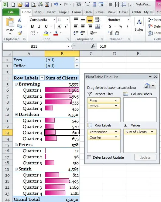
We’ll take a look at conditional formatting using a PivotTable that shows a schedule of 4 veterinarian appointments in a year. The table shows the number of clients by quarter and by location (farm or surgery).
To make the data more visual, I choose the values Farm (Farm) and Surgery (Surgery) of the first veterinarian with a surname Browning, i.e. cells from B6 to E7. With this range selected, I go to the tab Home (Home), press Conditional Formatting > Data Bars (Conditional Formatting > Bar Charts) and choose which color to use. These steps format the selected range so that a bar chart appears in each cell that shows the relative number of customers in each quarter and for each location.
In the following figure, we apply the format Data Bars (Histogram) to the first data range:
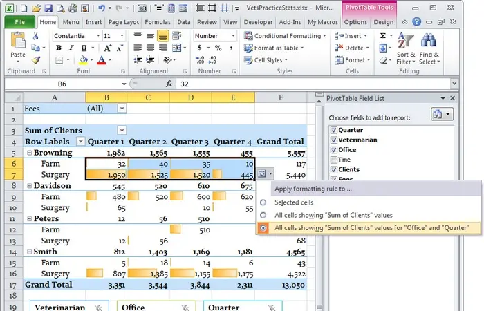
To apply the same formatting to similar data for other veterinarians, you need to select the previously formatted range, click the icon Formatting Options (Format Settings) that appears in the lower right corner of the range, and select the third of the options (see the figure below).
Thus, the rule will be applied to the same data of all other veterinarians in the summary table, without the need to apply this rule to each range individually. You can find the same options if you decide to create a new formatting rule in the dialog box New Formatting Rule (Create a formatting rule).
This figure shows how to apply the same conditional formatting to all data of the same type in our PivotTable:
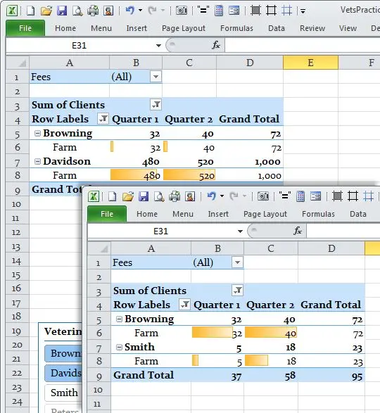
Now whenever you hide or show data while working with a PivotTable, the cell histograms will change to reflect the relative value of the value in each visible cell compared to all other visible cells of the same format.
Histograms change when the data in the pivot table changes, the length of the histogram depends on the data in all visible cells:
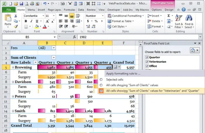
We can go even further and compare totals using a different formatting condition. In this case, I want to compare the totals for each veterinarian with the totals for the rest of the veterinarians, so I select cells from B5 to E5 – total number of clients (by quarters) of the veterinarian Browning. By creating histograms of a different color in this range, I can compare the totals of clients that were examined by a veterinarian Browning for those four blocks.
Like last time, the icon appears Formatting Options (Formatting Options), with which we can apply the same conditional formatting to the total data for each veterinarian’s clients.
Here you see histograms of a different color in cells with totals that can be visually compared with each other:
Other options
In some cases, it makes sense to separate conditional formatting, as was done in the previous example, applying it only to cells containing data of the same level, in order to separate totals and grand totals (Grand Total). But it doesn’t always make sense to do so.
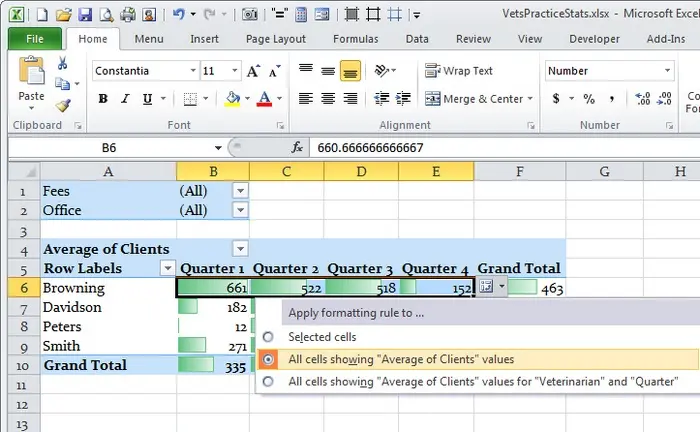
The data in the following pivot table shows the average number of customers, not the total number of customers, so you can apply the same conditional formatting to all cells in the table.
To do this, select the range B6: E6, let’s move on Conditional Formatting > Data Bars (Conditional Formatting > Histograms) and choose green color for the histograms. Next, in the formatting options, select the second option (see the figure below). The conditional formatting now covers both grand totals and grand totals, which, like all data in a pivot table, are averages. Therefore, it will not be a violation to compare them in the same way.
Here, all cells contain average values, so it is acceptable to apply one conditional formatting rule:
Moving data
Let’s go back to our original pivot table and start moving the data around. As you do this, you will notice that the formatting is saved in the right places. We moved the field Office (Place of reception) to the region report filters (Filters) and moved the field Quarter (Quarter) to region Row Labels (Rows), and at the same time all the purple histograms remained in their places.
Even if the table structure is changed and the fields are moved, the conditional formatting remains in place:
Restricted Formatting Rules
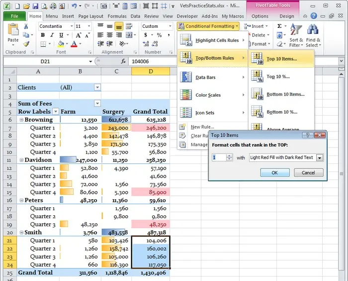
Of course, there are situations where you don’t want to apply conditional formatting to all ranges, but instead want to compare data within a narrower range. In our example, we want to see in which quarter each of our veterinarians performed best, regardless of location.
We will create a separate conditional formatting rule for each veterinarian’s quarterly totals, i.e. we need to highlight and apply the formatting to the cells D7: D10 (then D12:D15, then D17:D19 and so on). Then we use the rule Conditional Formatting > Top 10 Items (Conditional Formatting > First 10 Elements), set the condition for 1 cells, leave the default format. You can either copy this rule to an adjacent range, or create one for each individually.
To copy formatting, select one or more cells with the desired format and click Copy (Copy). Then select the range to which you want to copy the formatting, and on the tab Home (Home) select paste Special > Formats (Paste Special > Formats).
In some cases, you may want to compare data within a small area, rather than applying a conditional formatting rule to the entire group of non-contiguous ranges:
Conditional formatting in Excel, combined with the power of PivotTables, allows you to fine-tune the formatting and determine exactly what data to compare. You can compare similar with similar both across the entire pivot table and within one field that interests you. Knowing the options and knowing how to use them will help you compare values more clearly and get the desired result.