Conditional Formatting in Excel: Icon Sets

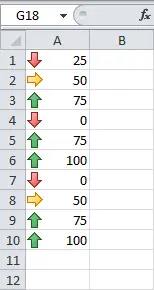
With icon sets in Excel 2010, it’s very easy to visualize cell values. Each icon represents a range of values.

To add an icon set, follow these steps:

1. Select a range of cells.
2. On the Advanced tab Home (Home) press the button Conditional Formatting > Icon sets (Conditional Formatting > Icon Sets) and select a subtype. Result:

   

   Explanation:

   • By default, for three icons, Excel calculates 67 and 33 percent of the maximum value in the range:

     67% = min + 0,67 * (max-min) = 2 + 0,67 * (95-2) = 64,31

     33% = min + 0,33 * (max-min) = 2 + 0,33 * (95-2) = 32,69

   • A green arrow will point to values ​​greater than or equal to 64,31.
   • The yellow arrow will point to values ​​that are greater than or equal to 32,69 but less than 64,31.
   • A red arrow will appear next to values ​​less than 32,69.
3. Change the values. Result: Excel automatically updates the icon set.

Read on to learn how to customize the icon set.

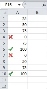
4. Highlight a range A1: A10.
5. On the Advanced tab Home (Home) press the button Conditional Formatting > Rule management (Conditional Formatting > Manage Rules).
6. Выберите Ofchange the rule (Edit rule).Excel will display a dialog box Change a formatting rule (Edit Formatting Rule). Here you can customize the icon set by changing the following options: Icon style (Icon Style), Reverse icon order (Reverse Icon Order), Show icon only (Show Icon Only), Icon (Icon), Value (Value), A type (Type) etc.

Note: To open this dialog box for new rules, on the 2nd step of our instructions, click Other rules (More Rules).

7. From drop down list Icon style (Icon Style) select 3 symbols without circles. In the drop-down menu of the second icon, click on No cell icon (No Cell Icon). In both fields A type (Type) establish Number (Number) and replace the values ​​with 100 and 0 respectively. Select symbol “>» from the drop-down list next to the value 0 (see figure below).
8. Double tap OK.Result: