Conditional Formatting in Excel: Color Scales

Color scales in Excel 2010 make it very easy to visualize values ​​in a range of cells. The tint of the color shows the value in the cell.

To add a color scale, follow our instructions:

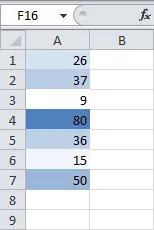
1. Select a range of cells.
2. On the Advanced tab Home (Home) press the button Conditional Formatting > Color scales (Conditional Formatting > Color Scales) and select a subtype. Result:

   

   Explanation:

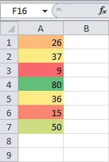
   • By default, for a three-color scale, Excel calculates the 50th percentile (same as the median or mean).
   • The cell that contains the minimum value (9) is red.
   • The cell containing the average value (36) is yellow.
   • The cell with the maximum value (80) is colored green.
   • All other cells are colored proportionally.

Read on to learn how to customize the color bar.

3. Highlight a range A1: A7.
4. On the Advanced tab Home (Home) press the button Conditional Formatting > Rule management (Conditional Formatting > Manage Rules).
5. Click on treasonread the rule (Edit rule).Excel will display a dialog box Change a formatting rule (Edit Formatting Rule). Here you can customize the color scale by changing the following options: Format style (Format Style), The minimum value (Minimum), Average and maximum value (Midpoint and Maximum), Color (Color) etc.

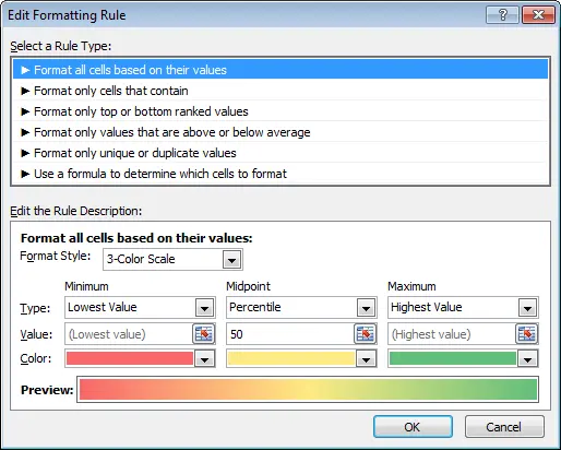
Note: To open this dialog box for new rules, on the 2nd step of our instructions, click Other rules (More Rules).

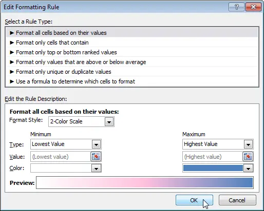
6. Set the two-color scale in the dropdown Format style (Format Style) and choose white and blue colors.
7. Double tap OK.Result: