Coloring alternating rows in Excel

This example will demonstrate how to use conditional formatting to fill in alternating lines. Coloring every other line in a range will make your data more readable.

1. Select a range.
   
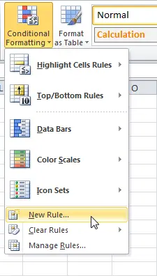
2. On the Advanced tab Home (Home) press the button Conditional Formatting > Create Rule (Conditional Formatting > New Rule).
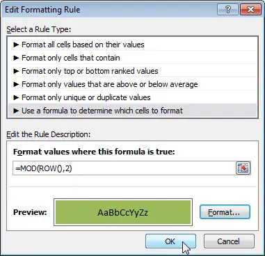
3. Выберите Use a formula to determine which cells to format (Use a formula to determine which cells to format).
4. Enter the following formula:

   =MOD(ROW(),2)

   =ОСТАТ(СТРОКА();2)

5. Define the formatting style and click OK.

   Result:

   

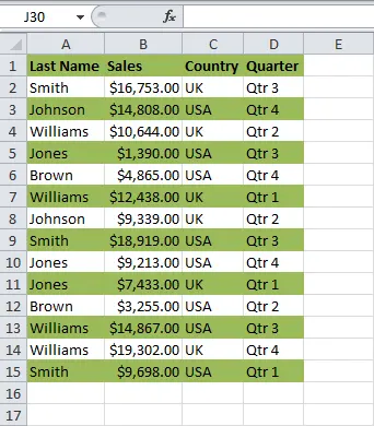
   Explanation:

   • Function LINE (ROW) returns the row number.
   • Function THE REST (MOD) returns the remainder of a division. For example, in the seventh row, MOD(7;2) is 1 because 7 is divisible by 2 (3 times) with a remainder of 1. For the eighth row, MOD(8;2) is 0 because 8 is divisible by 2 (exactly 4 times) and gives a remainder of 0.
   • As a result, all odd rows return 1, i.e. TRUE (TRUE), and are painted over in the specified color.