Calculate Percentage of Number and Share in Excel

Interest calculations are one of the most popular actions performed in Excel. This can be multiplying a number by a certain percentage, determining the share (in%) of a specific number, etc. However, even if the user knows how to perform calculations on a piece of paper, he cannot always repeat them in the program. Therefore, now, we will analyze in detail how interest is calculated in Excel.

We count the share of the total number

To begin with, let’s analyze a fairly common situation when we need to determine the proportion of one number (as a percentage) in another. The following is a mathematical formula for performing this task:

Share (%) = Number 1/Number 2*100%, where:

• Number 1 – in fact, our original numerical value
• The number 2 is the final number in which we want to find out the share

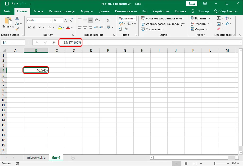
For example, let’s try to calculate what is the proportion of the number 15 in the number 37. We need the result as a percentage. In this, the value of “Number 1” is 15, and “Number 2” is 37.

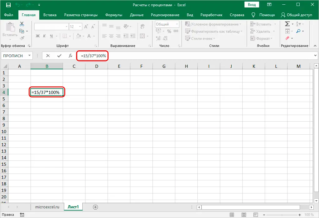
1. Select the cell where we need to make calculations. We write the “equal” sign (“=”) and then the calculation formula with our numbers: =15/37*100%.
2. After we have typed the formula, we press the Enter key on the keyboard, and the result will immediately be displayed in the selected cell.

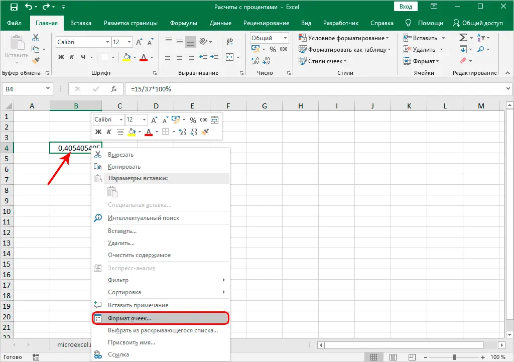
For some users, in the resulting cell, instead of a percentage value, a simple number may be displayed, and sometimes with a large number of digits after the decimal point.

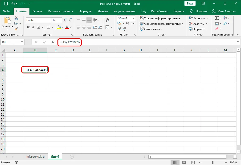
The thing is that the cell format for displaying the result is not configured. Let’s fix this:

1. We right-click on the cell with the result (it doesn’t matter before we wrote the formula in it and got the result or after), in the list of commands that appears, click on the “Format Cells…” item.
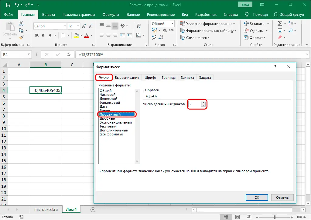
2. In the formatting window, we will find ourselves in the “Number” tab. Here, in numerical formats, click on the line “Percentage” and in the right part of the window indicate the desired number of decimal places. The most common option is “2”, which we set in our example. After that, press the OK button.
3. Done, now we will get exactly the percentage value in the cell, which was originally required.

By the way, when the display format in a cell is set as a percentage, it is not at all necessary to write “* 100%“. It will be enough to perform a simple division of numbers: =15/37.

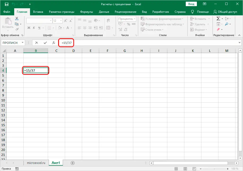
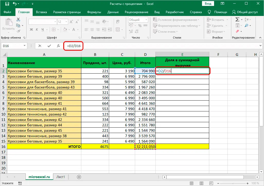
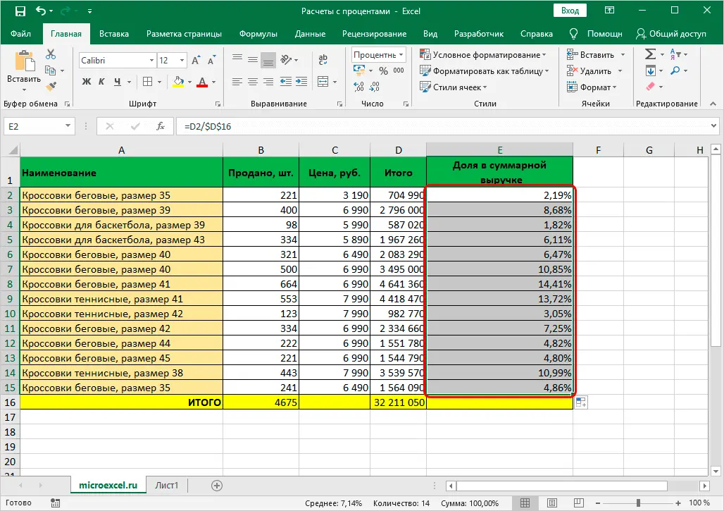
Let’s try to apply the acquired knowledge in practice. Let’s say we have a table with sales by various items, and we need to calculate the share of each product in the total revenue. For convenience, it is better to display the data in a separate column. Also, we must have pre-calculated the total revenue for all items, by which we will divide sales for each product.

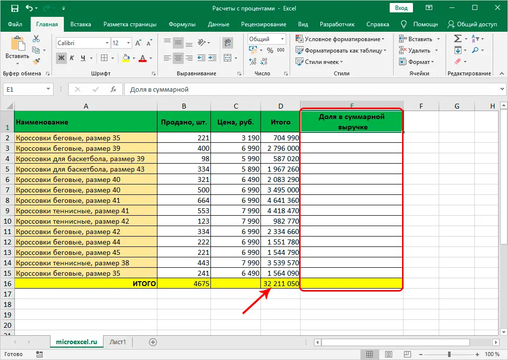
So, let’s get down to the task at hand:

1. Select the first cell of the column (excluding the table header). As usual, the writing of any formula begins with the sign “=“. Next, we write a formula for calculating the percentage, similar to the example considered above, only replacing specific numerical values ​​with cell addresses that can be entered manually, or adding them to the formula with mouse clicks. In our case, in a cell E2 you need to write the following expression: =D2/D16. Note: do not forget to pre-configure the cell format of the resulting column by choosing to display as percentages.
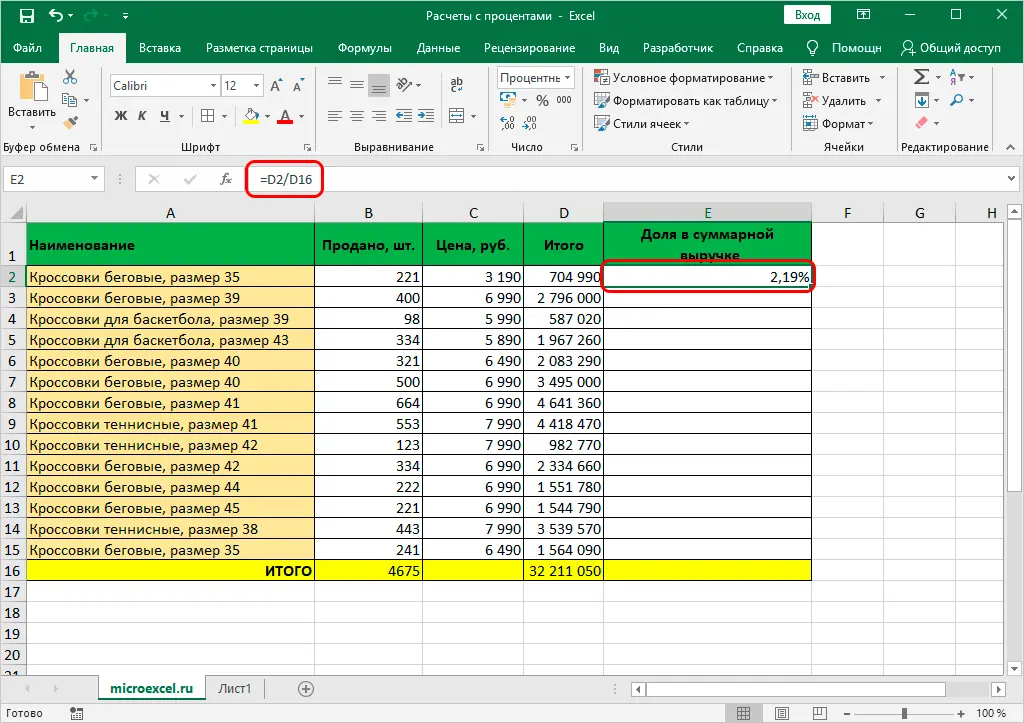
2. Press Enter to get the result in the given cell.
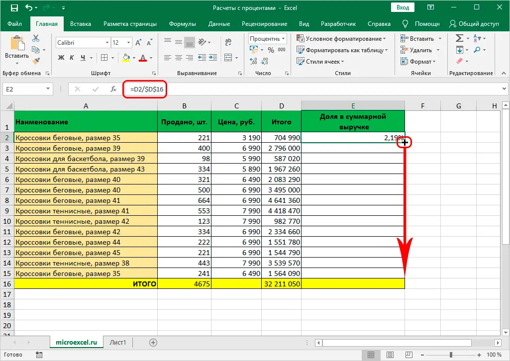
3. Now we need to make similar calculations for the remaining rows of the column. Fortunately, Excel’s capabilities allow you to avoid manually entering the formula for each cell, and this process can be automated by copying (stretching) the formula to other cells. However, there is a small nuance here. In the program, by default, when copying formulas, cell addresses are adjusted according to the offset. When it comes to sales of each individual item, it should be so, but the coordinates of the cell with the total revenue should remain unchanged. To fix it (make it absolute), you need to add the symbol “$“. Or, in order not to type this sign manually, by highlighting the cell address in the formula, you can simply press the key F4. When finished, press Enter.
4. Now it remains to stretch the formula to other cells. To do this, move the cursor to the lower right corner of the cell with the result, the pointer should change shape to a cross, after which, stretch the formula down by holding down the left mouse button.
5. That’s all. As we wanted, the cells of the last column were filled with the share of sales of each specific product in total revenue.

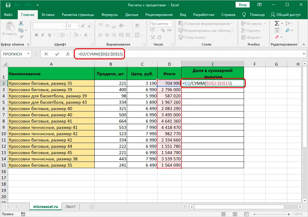
Of course, in the calculations it is not at all necessary to calculate the final revenue in advance and display the result in a separate cell. Everything can be immediately calculated using one formula, which for a cell E2 look like this: =D2/СУММ(D2:D15).

In this case, we immediately calculated the total revenue in the share calculation formula using the function SUM. Read about how to apply it in our article – ““.

As in the first option, we need to fix the figure for the final sales, however, since a separate cell with the desired value does not take part in the calculations, we need to put down the signs “$” before the designations of rows and columns in the cell addresses of the sum range: =D2/СУММ($D$2:$D$15).

Finding a percentage of a number

Now let’s try to calculate the percentage of a number as an absolute value, i.e. as a different number.

The mathematical formula for the calculation is as follows:

Number 2 = Percentage (%) * Number 1, where:

• The number 1 is the original number, the percentage for which you want to calculate
• Percentage – respectively, the value of the percentage itself
• The number 2 is the final numeric value to be obtained.

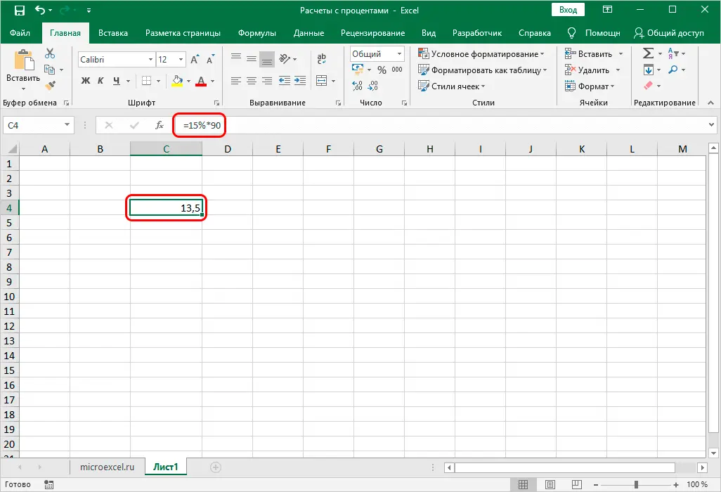
For example, let’s find out what number is 15% of 90.

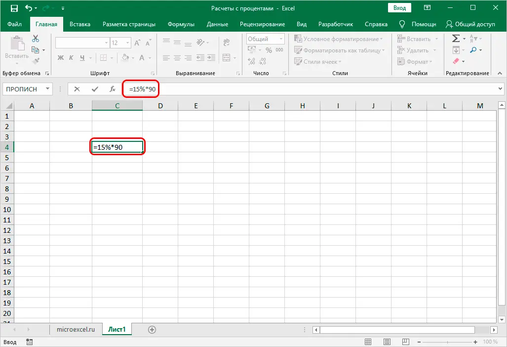
1. We select the cell in which we will display the result and write the formula above, substituting our values ​​into it: =15%*90.Note: Since the result must be in absolute terms (i.e. as a number), the cell format is “general” or “numeric” (not “percentage”).
2. Press the Enter key to get the result in the selected cell.

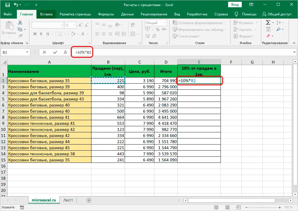
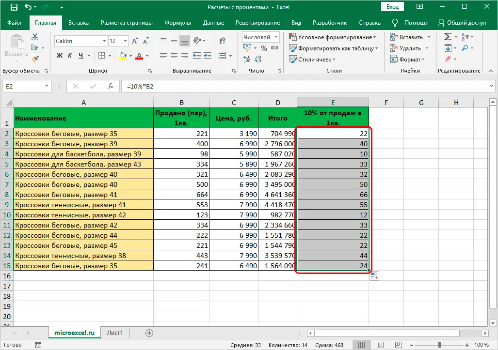
Such knowledge helps to solve many mathematical, economic, physical and other problems. Let’s say we have a table with shoe sales (in pairs) for 1 quarter, and we plan to sell 10% more next quarter. It is necessary to determine how many pairs for each item correspond to these 10%.

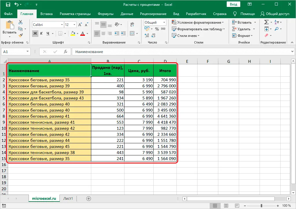
To complete the task, follow these steps:

1. For convenience, we create a new column, in the cells of which we will display the results of calculations. Select the first cell of the column (counting the headers) and write the formula above in it, replacing the specific value of a similar number with the cell address: =10%*B2.
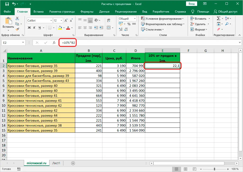
2. After that, press the Enter key, and the result will immediately be displayed in the cell with the formula.
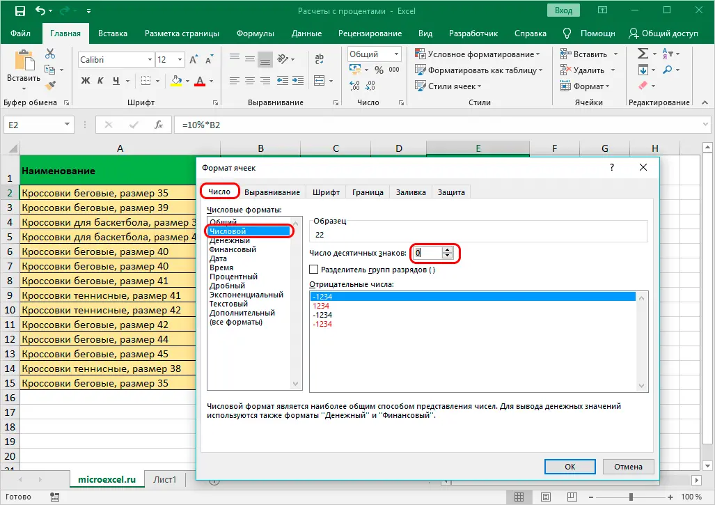
3. If we want to get rid of the digits after the decimal point, since in our case the number of pairs of shoes can only be calculated as integers, we go to the cell format (we discussed how to do this above), where we select a numeric format with no decimal places.
4. Now you can extend the formula to the remaining cells in the column.

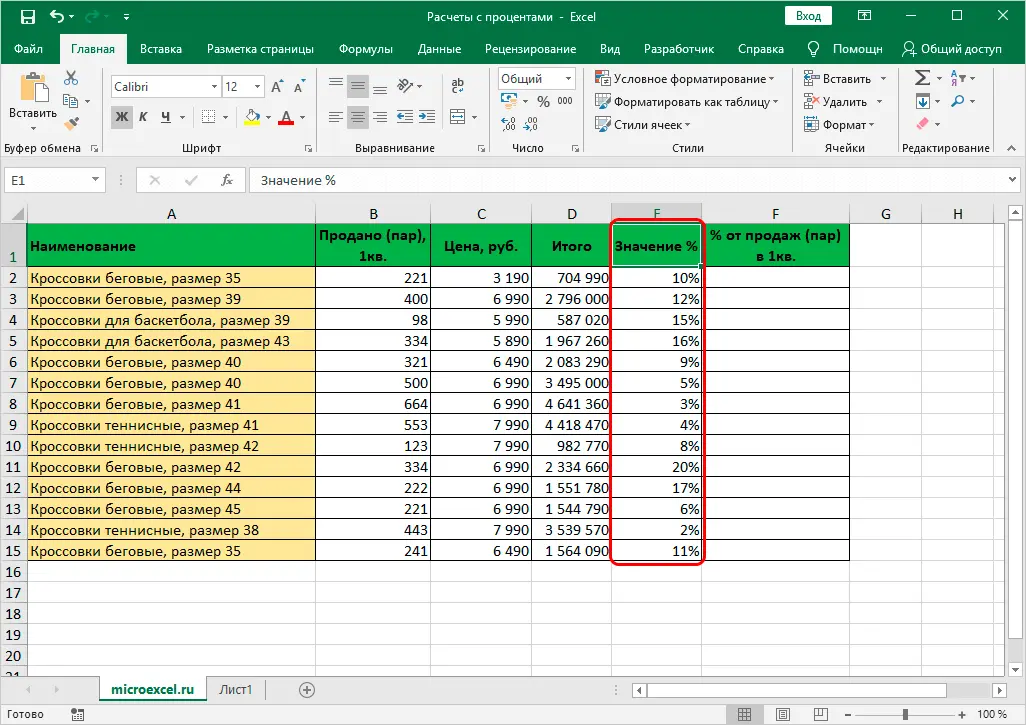
In cases where we need to get different percentages from different numbers, accordingly, we need to create a separate column not only for displaying the results, but also for the percentage values.

1. Let’s say our table contains such a column “E” (Value %).
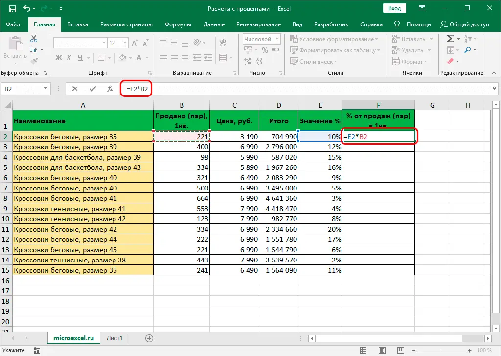
2. We write the same formula in the first cell of the resulting column, only now we change the specific percentage value to the address of the cell with the percentage value contained in it: =E2*B2.
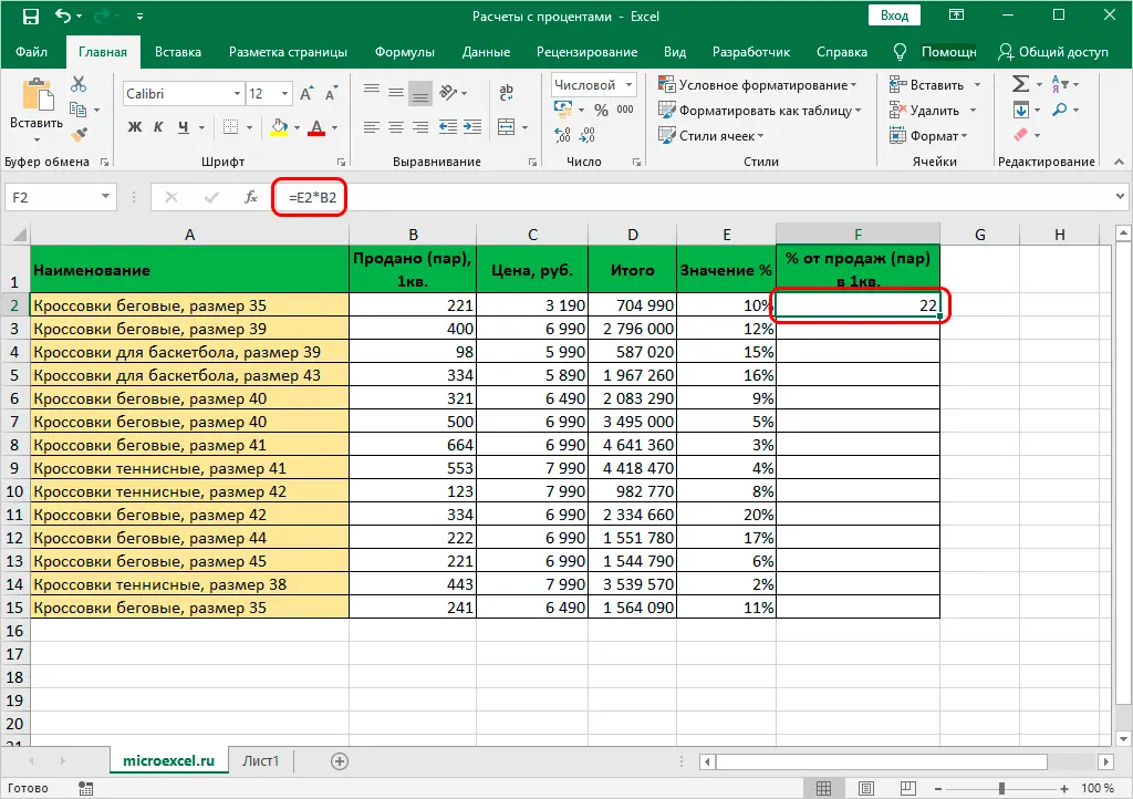
3. By clicking Enter we get the result in the given cell. It remains only to stretch it to the bottom lines.

Conclusion

While working with tables, it is often necessary to make calculations with percentages. Fortunately, the functionality of the Excel program allows you to perform them with ease, and if we are talking about the same type of calculations in large tables, the process can be automated, which will save a lot of time.