Contents
Formulation of the problem
As input data, we have an Excel file, where one of the sheets contains several tables with sales data of the following form:
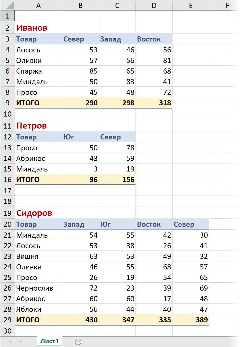
Note that:
- Tables of different sizes and with different sets of products and regions in rows and columns without any sorting.
- Blank lines can be inserted between tables.
- The number of tables can be any.
Two important assumptions. It is assumed that:
- Above each table, in the first column, there is the name of the manager whose sales the table illustrates (Ivanov, Petrov, Sidorov, etc.)
- The names of goods and regions in all tables are written in the same way – with a case accuracy.
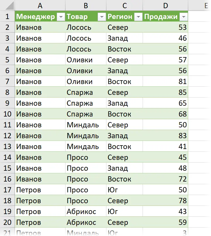
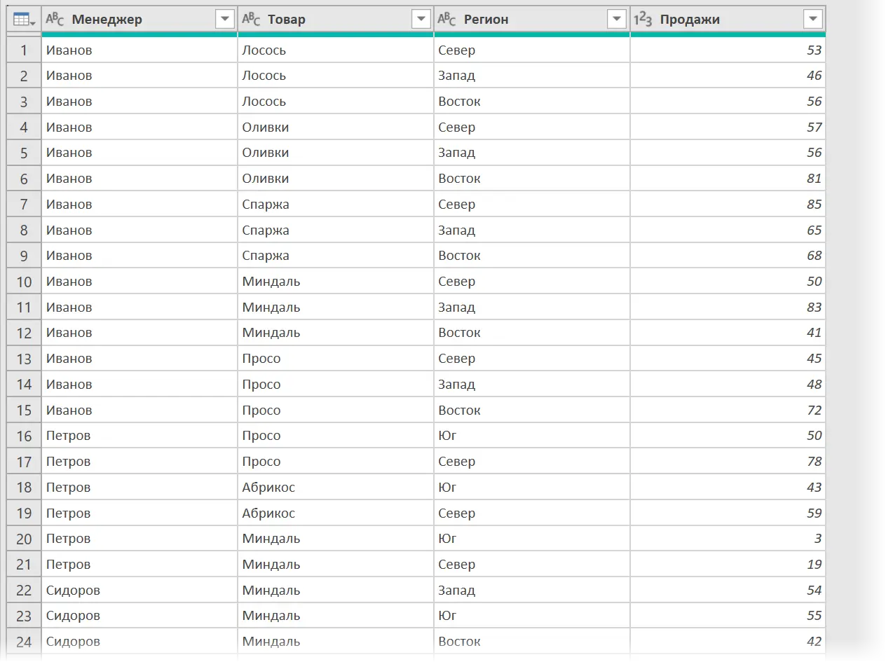
The ultimate goal is to collect data from all tables into one flat normalized table, convenient for subsequent analysis and building a summary, i.e. in this one:
Step 1. Connect to the file
Let’s create a new empty Excel file and select it on the tab Data Command Get Data – From File – From Book (Data — From file — From workbook). Specify the location of the source file with sales data and then in the navigator window select the sheet we need and click on the button Convert Data (Transform Data):
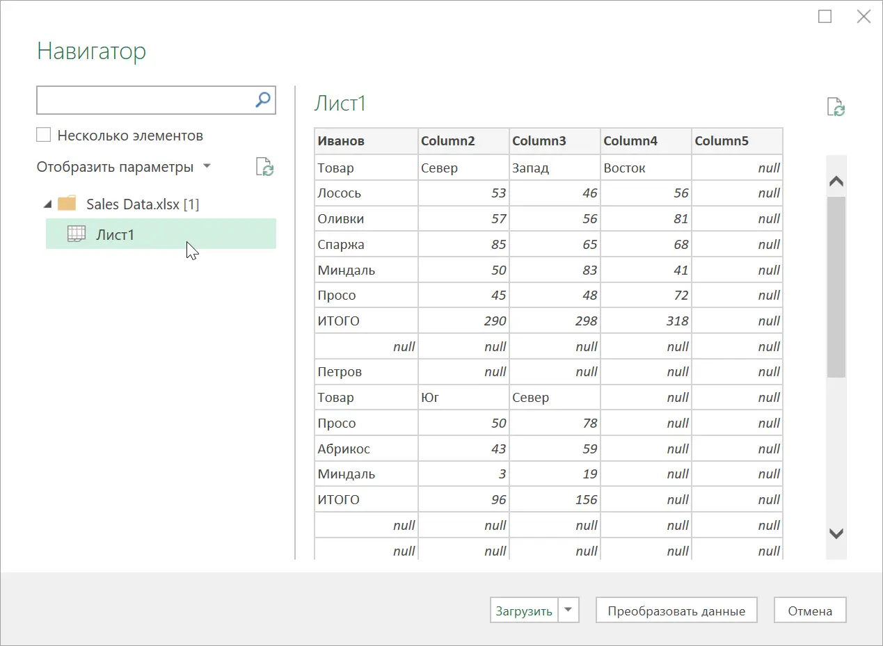
As a result, all data from it should be loaded into the Power Query editor:
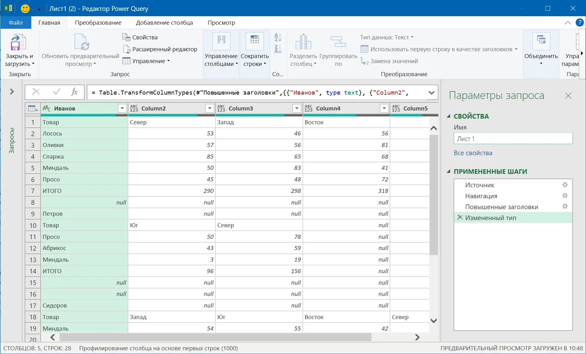
Step 2. Clean up the trash
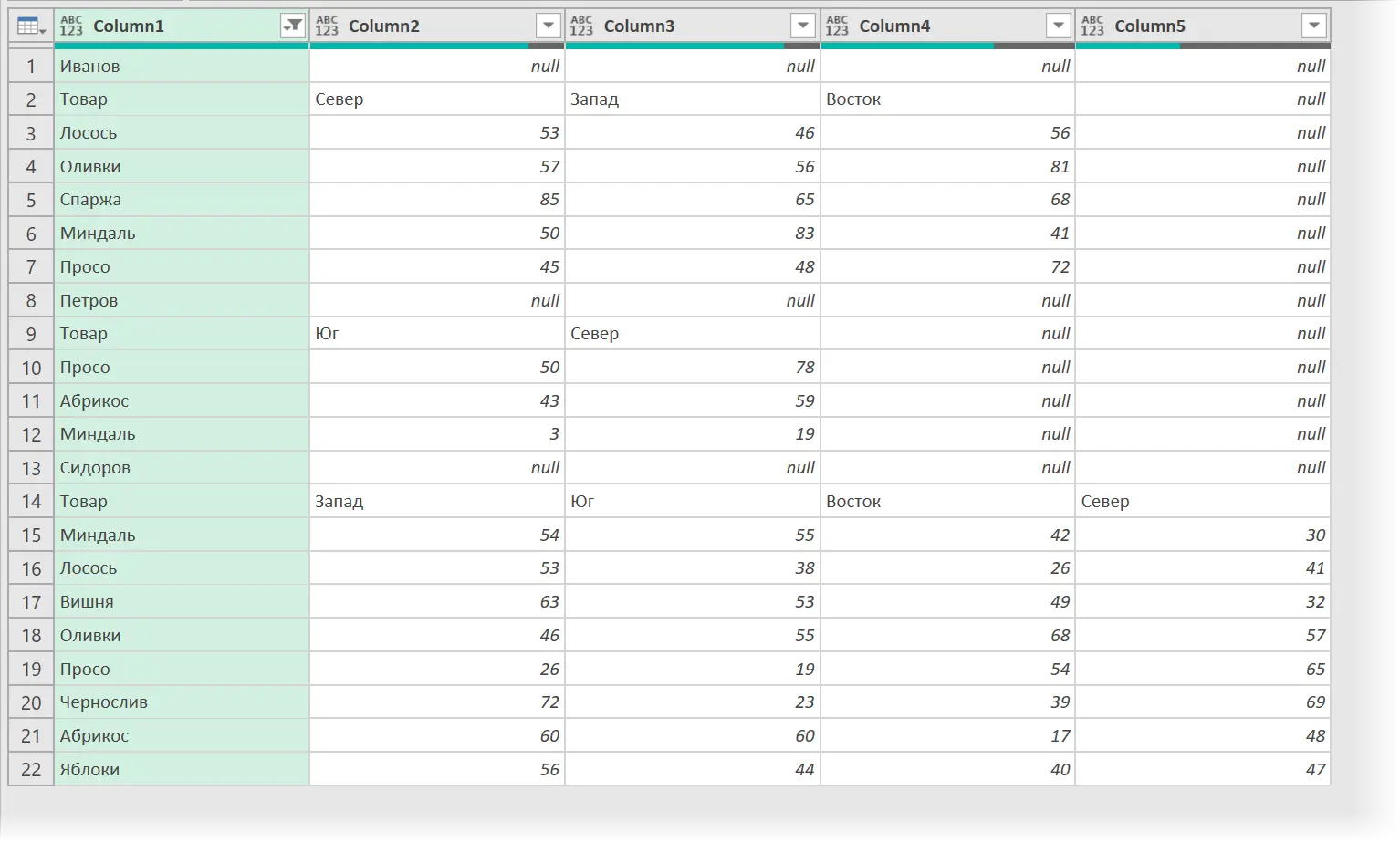
Delete automatically generated steps modified type (Changed Type) и Elevated headers (Promoted Headers) and get rid of empty lines and lines with totals using a filter null и TOTAL by the first column. As a result, we get the following picture:
Step 3. Adding managers
In order to understand later where whose sales are, it is necessary to add a column to our table, where in each row there will be a corresponding surname. For this:
1. Let’s add an auxiliary column with line numbers using the command Add Column – Index Column – From 0 (Add column — Index column — From 0).
2. Add a column with a formula with the command Adding a Column – Custom Column (Add column — Custom column) and introduce the following construction there:
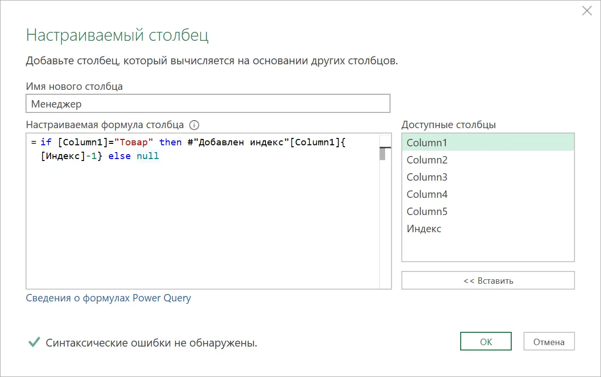
The logic of this formula is simple – if the value of the next cell in the first column is “Product”, then this means that we have stumbled upon the beginning of a new table, so we display the value of the previous cell with the name of the manager. Otherwise, we do not display anything, i.e. null.
To get the parent cell with the last name, we first refer to the table from the previous step #”Index added”, and then specify the name of the column we need [Column1] in square brackets and the cell number in that column in curly brackets. The cell number will be one less than the current one, which we take from the column Index, respectively.
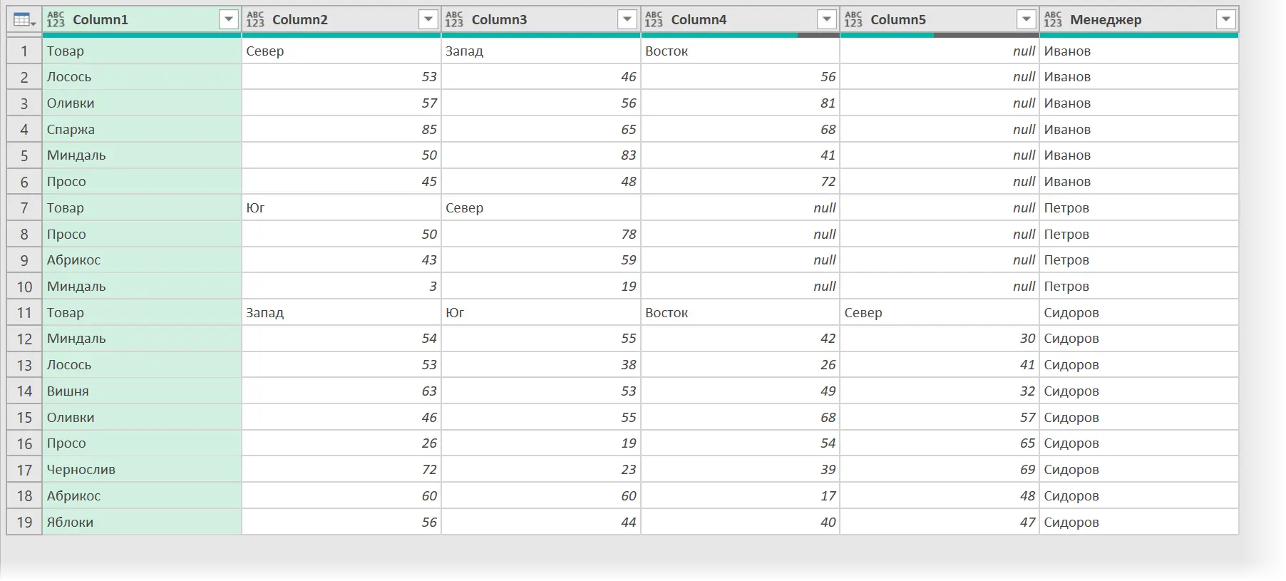
3. It remains to fill in the empty cells with null names from higher cells with the command Transform – Fill – Down (Transform — Fill — Down) and delete the no longer needed column with indices and rows with last names in the first column. As a result, we get:
Step 4. Grouping into separate tables by managers
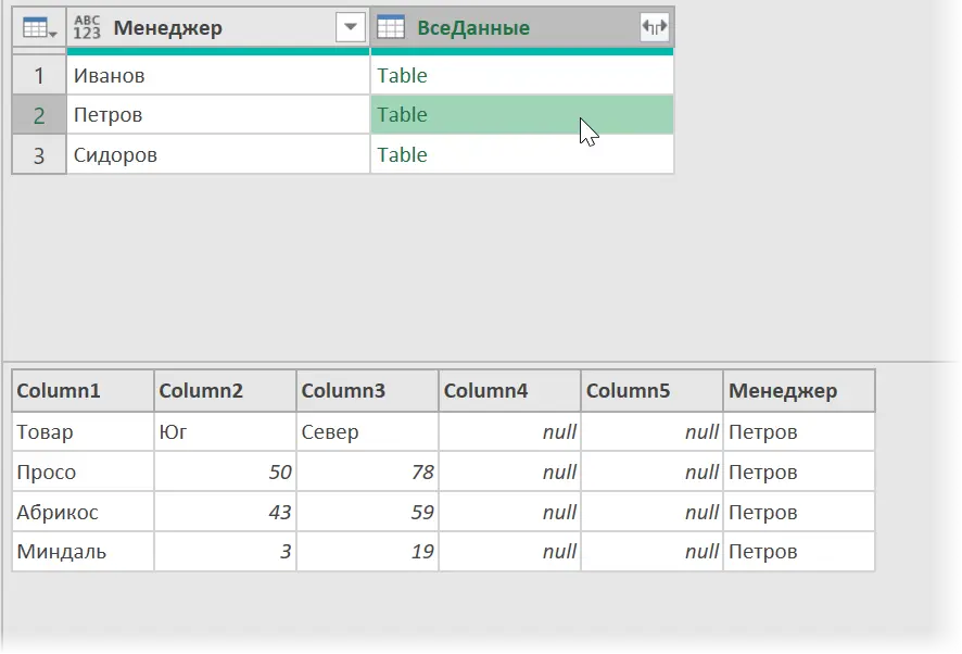
The next step is to group the rows for each manager into separate tables. To do this, on the Transformation tab, use the Group by command (Transform – Group By) and in the window that opens, select the Manager column and the operation All rows (All rows) to simply collect data without applying any aggregating function to them (sum, average, etc.). P.):

As a result, we get separate tables for each manager:
Step 5: Transform Nested Tables
Now we give the tables that lie in each cell of the resulting column All data in decent shape.
First, delete a column that is no longer needed in each table Manager. We use again Custom column tab Transformation (Transform — Custom column) and the following formula:
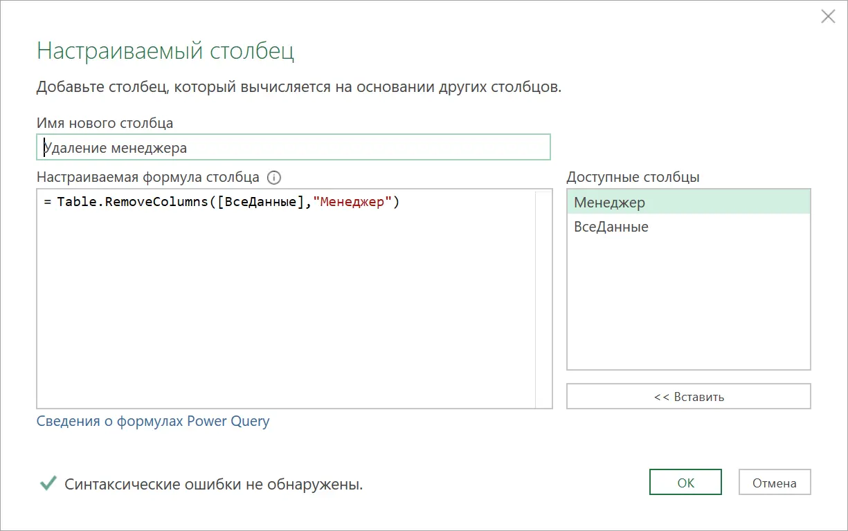
Then, with another calculated column, we raise the first row in each table to the headings:
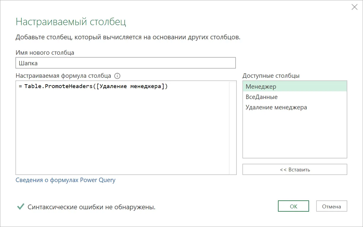
And finally, we perform the main transformation – unfolding each table using the M-function Table.UnpivotOtherColumns:
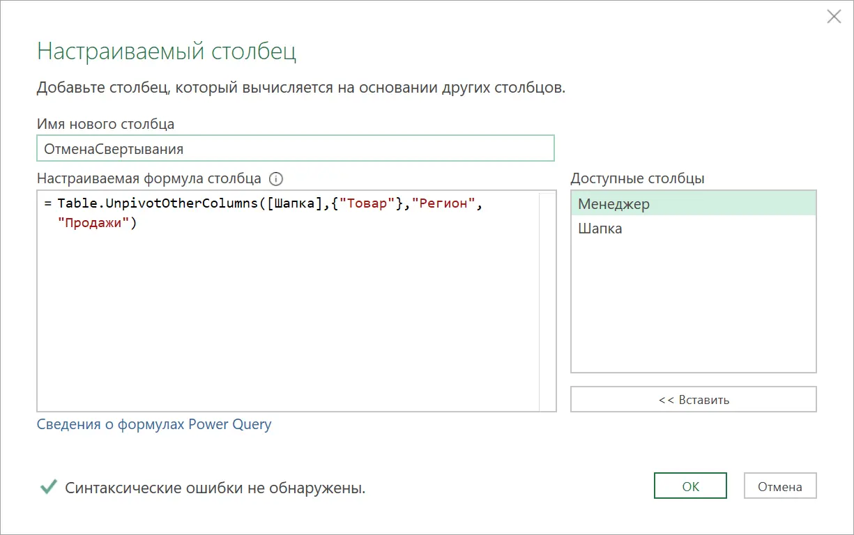
The names of the regions from the header will go into a new column and we will get a narrower, but at the same time, a longer normalized table. Empty cells with null are ignored.
Getting rid of unnecessary intermediate columns, we have:
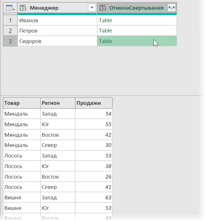
Step 6 Expand Nested Tables
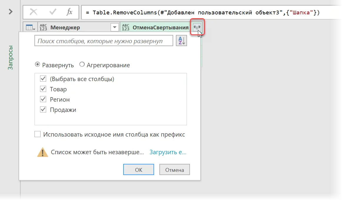
It remains to expand all normalized nested tables into a single list using the button with double arrows in the column header:
… and we finally get what we wanted:
You can export the resulting table back to Excel using the command Home — Close and Load — Close and Load in… (Home — Close&Load — Close&Load to…).
- Build tables with different headers from multiple books
- Collecting data from all files in a given folder
- Collecting data from all sheets of the book into one table


