Building a Bubble Chart in Excel

In Microsoft Office Excel, you can create various charts from the original table array. They allow you to visually assess the situation, compare the parameters in the table, draw the appropriate analysis and conclusions. In this article, we will talk about building a bubble (scatter) chart in Excel.

How to build a bubble chart without animation

On such a graph, the bubbles will not move in worksheet space, i.e. the image will look flat. To make such a diagram, you must follow the following algorithm of actions:

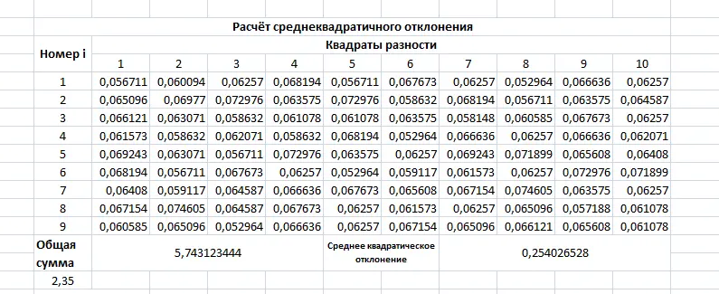
1. In the constructed table, use the left key of the manipulator to select the values ​​that need to be compared and displayed on the graph.

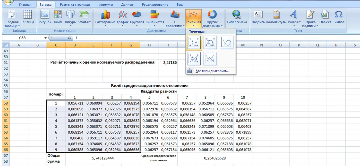
2. In the upper toolbar of the program, go to the “Insert” section.
3. Expand the area with chart options and select the bubble one by clicking on it with LMB. All graphs are presented schematically in the selection box.

4. Check result. A bubble chart without animation will appear next to the plate, reflecting the values ​​of the initial values.

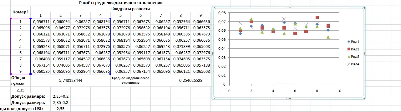
Pay attention! If desired, some values ​​on the resulting graph can be changed. For example, axis labels, scale, title. You can also add an additional chart for other columns of the table, aligning it with the one you created.

How to create an interactive bubble chart in Excel

This method is more complicated than the previous one in terms of implementation, however, it gives a more accurate idea of ​​the ongoing processes, guided by tabular values. To build this type of chart, you need to follow simple steps according to the instructions:

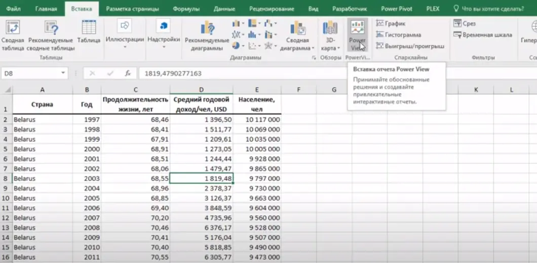
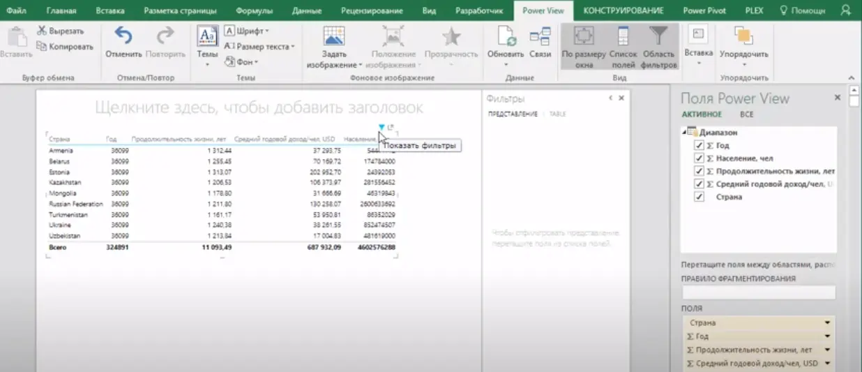
1. Open a Power View sheet. This is a special Microsoft Office Excel add-in that first appeared in the 2013 version. Therefore, on earlier versions of the software, this method will not work. To start, you need to click on the “Power View” button located in the “Insert” section next to the overviews function.

2. Wait for the Power View sheet to open. This procedure may take several seconds. In the launched add-in, you can immediately close the filter menu, which is not needed to build a chart.
3. On the right side of the tool that opens, the names of the columns of the source table will be presented. If these headings are unchecked, then the table located in the center of the slide will also change.

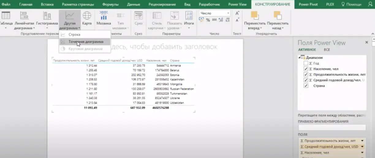
4. From the constructed table itself in Power View, you can make a bubble chart. To do this, at the top of the main menu of the tool, you need to enter the “Design” section, and then expand the “Other diagram” subsection by clicking on the arrow below.
5. In the drop-down list of options, click on the word “Scatter Plot”. This is the bubble, only here it is called differently.

6. Analyze the result. Now the original table array will turn into a bubble chart. It can be scaled up if desired.

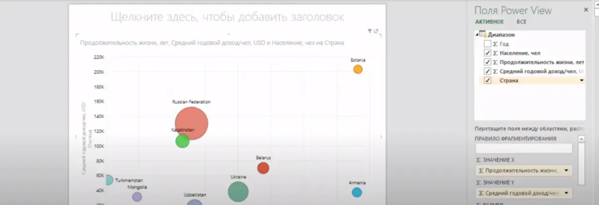
7. If the axes in the chart are named incorrectly, then this can be corrected in the toolbar on the right side of the Power View window by dragging the desired titles to the “Slicing Rule” section and swapping them.
8. In order for the constructed chart to become animated and be able to move the bubbles around the working field, showing the development of the situation in time, you must enable the “Reproduction Axis” section in the same “Fragmentation Rule” area in the right Power View menu. In this axis, you should drag the name of the desired axis from the constructed chart.

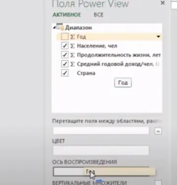
9. After completing the previous steps, an additional time axis will be added to the chart, and the “Play” button will appear next to the selected axis, after clicking on which the bubbles will begin to move in space.

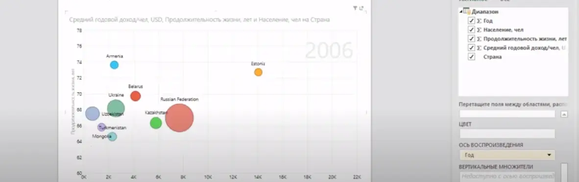
Important! Each “bubble” in the scatter plot has its own name, which also moves as it moves. The size of the titles can be changed directly on the chart itself.

How to consider a single element in a scatter plot like

In Microsoft Office Excel, there is such a possibility. Those. to study the behavior of a particular characteristic on a bubble chart, it must be isolated and analyzed. The selection process is divided into several stages, each of which should be considered in detail to fully understand the topic:

1. Build a scatter plot and start the animation of its elements according to the above scheme.
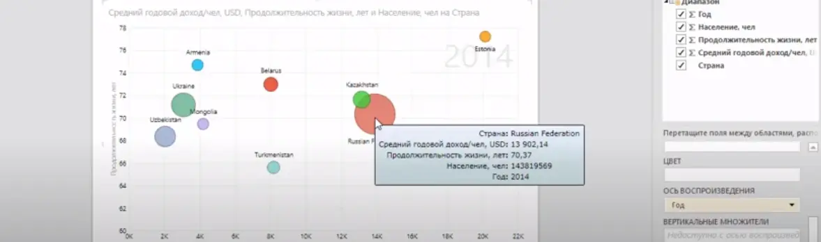
2. Move the mouse cursor over the “bubble” that requires detailed study. After that, a dialog box with detailed information about it will be displayed next to the selected element.

3. With the left mouse button, click once on this element. The trajectory of its movement will be shown on the chart.
4. Click on the “Play” button. Now only the selected “bubble” will move along the diagram, and the user will be able to examine its behavior in more detail.

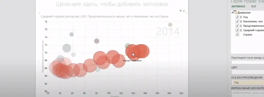
As the bubbles move, a horizontal bar will move from the bottom of the chart. When it reaches the leftmost position, the animation will stop. A similar approach can be used for countries, company visualization, product development, affiliates, competition, evaluation of product quality indicators, business processes, etc. The general principle of constructing a scatter plot will not change.

Additional Information! When creating an animated scatter plot in the Power View add-in, the user can set the time and speed at which the graded items move.

Conclusion

Thus, it is not difficult to build a scatter plot in Excel, knowing the basic principle of its creation and acting on the algorithm discussed above.