


After reading this article, you will learn how to use array formulas. It should be noted that they perform several calculations in one cell. This is very convenient: now you do not have to create bulky tables for less complex calculations.
Application of the conventional method
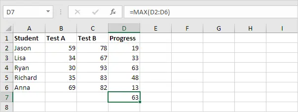
To find the indicators in the Progress column, we need to follow the following instruction:
- To begin with, we will determine the performance of each student.
- Then we apply the function MAX() to determine the maximum score in the Progress column.

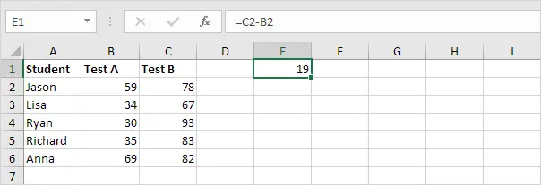
Calculation with an array formula
When using an array formula, there is no need to create an additional “D” column. The program itself will remember all the intermediate data. The information stored in “memory” is called “Array of constants”.
- So, to determine the progress of the first student, you need to use the formula presented in the screenshot below.

- To determine the maximum indicator, you need to apply the function MAX() and replace C2 with the range C2:C6 and B2 with B2:B6.
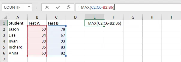
- Finish creating the function by pressing CTRL + SHIFT + ENTER.
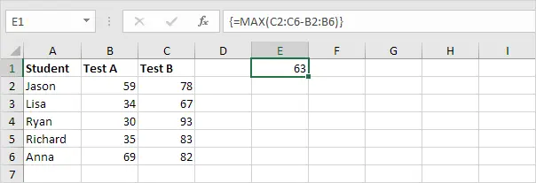
Note: array formulas are always delimited by curly braces. Do not enter them yourself as they will disappear.
Explanation: The array constant is stored in the Excel data store. She looks like this:
{19; 33; 63; 48; 13}
We use this constant as a variable in the function MAX(), so we end up with 63.
Using the F9 Key
If necessary, you can view the entire contents of the array of constants.
- Specify C2:C6-B2:B6 in the formula.
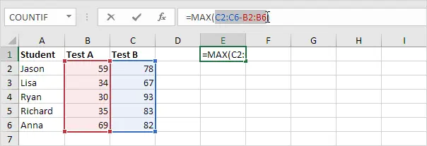
- Press the F9 key.
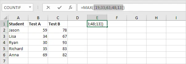
Ready! You may notice that the values of the vertical array are separated by a semicolon, while the data of the horizontal array is simply separated by a comma.