


Contents
This tutorial provides practical examples of using array formulas in Excel. This is the bare minimum that can be done with them. I hope that most of these examples will definitely come in handy for solving your everyday problems.
Counting the number of characters in a range of cells
The figure below shows a formula that counts the number of characters, including spaces, in the range A1:A10.
In this example, the function DLSTR counts the length of each text string from the given range, and the function SUM – sums these values.
Largest and smallest range values in Excel
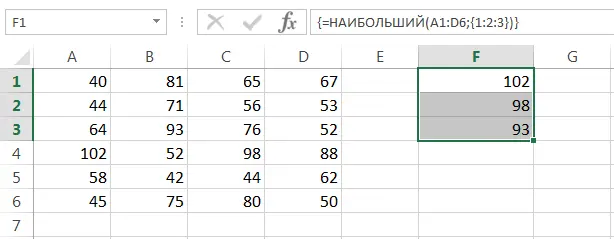
The following formula returns the 3 largest values in the range A1:D6
To return a different number of largest values, just change the array of constants. For example, the following formula already returns the 6 largest values in the same range:
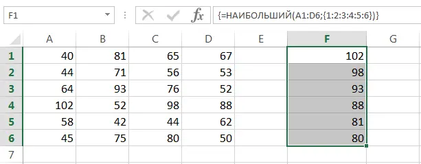
If you need to find the smallest values, just replace the function LARGE on LEAST.
Counting the number of differences between two ranges in Excel
The array formula shown in the figure below allows you to count the number of differences in two ranges:
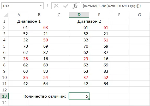
This formula compares the corresponding values of two ranges. If they are equal, the function IF returns zero, and if not equal – one. The result is an array that consists of zeros and ones. Then the function SUM sums the values of the given array and returns the result.
It is required that both ranges being compared have the same size and orientation.
Transposing an array in Excel
Recall the previous example and try to complicate the task. For example, you want to compare ranges in Excel that are the same size but have different orientations—one is horizontal and the other is vertical. In this case, the TRANSPOSE function will come to the rescue, which allows you to transpose an array. Now the formula from the previous example will get a little more complicated:
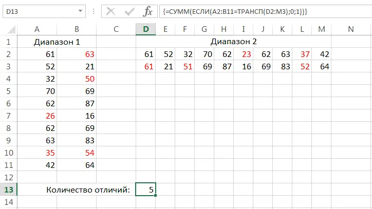
Transposing an array in Excel means changing its orientation, or rather, replacing rows with columns and columns with rows.
Sum rounded values in Excel
The figure below shows the goods, the price of which is indicated in euros, as well as their quantity and the total cost in rubles. Cell D9 displays the total amount of the entire order.
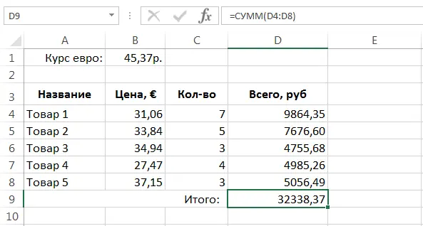
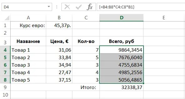
If you change the formatting in the range D4:D8, it becomes clear that the values in these cells are not rounded, but just visually formatted. Accordingly, we cannot be sure that the amount in cell D9 is accurate.
In Excel, there are at least two ways to correct this error.
- Enter already rounded values in cells D4:D8. The array formula would look like this:
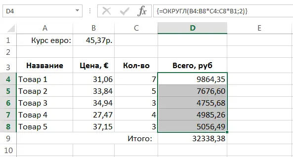

- Use an array formula in cell D9 that first rounds the values and then sums them.
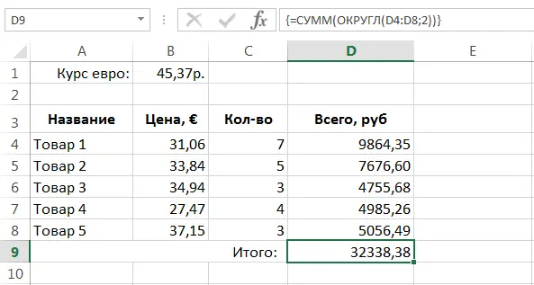
Now we can be sure that the amount in cell D9 is correct.
As you can see, the amount before and after rounding is slightly different. In our case, this is just one penny.
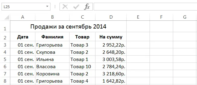
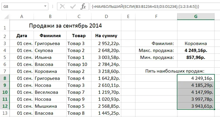
Maximum or minimum value by condition
The figure below shows a fragment of the sales table, in which there are 1231 positions. Our task is to calculate the maximum sale that a given seller made.
Let in cell G3 we will set the name of the seller, then the array formula will look like this:
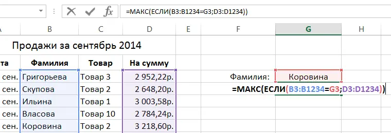
In this case, the function IF compares the values in the range B3:B1234 with the given last name. If the names match, then the amount of the sale is returned, and if not, LYING. As a result, the function IF generates a one-dimensional vertical array, which consists of the sums of sales of the specified seller and the values LYING, total 1231 positions. Then the function MAX processes the resulting array and returns the maximum sale from it. In our case, this is:
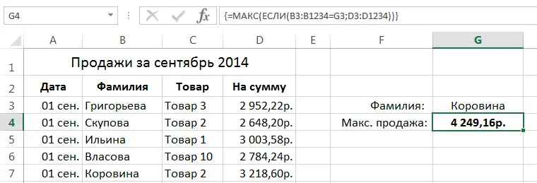
If the array contains boolean values, then the functions MAX и MIN they are ignored.
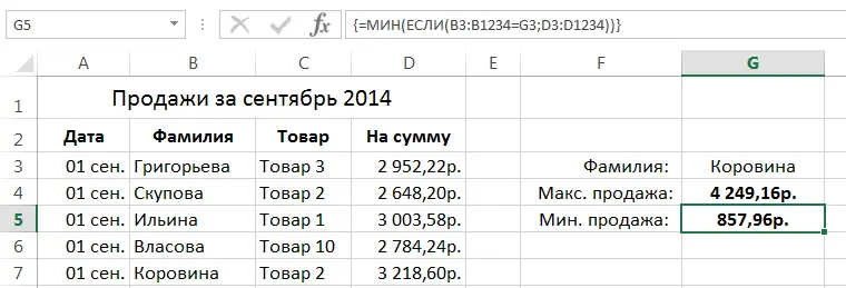
To derive the minimum sale, use this formula:
This formula allows you to display the 5 highest sales of the specified seller:
So, in this lesson, we looked at some interesting examples of using array formulas in Excel. I hope that they were useful for you and will definitely come in handy in the future. For more information about arrays, read the following articles:
- Introduction to array formulas in Excel
- Multicell array formulas in Excel
- Single cell array formulas in Excel
- Arrays of constants in Excel
- Editing array formulas in Excel
- Approaches to editing array formulas in Excel