


Contents
This tutorial explains how to set up alternate row fill colors and automatically highlight every second row or column in a worksheet. You will learn how to create alternating rows and columns in Excel, as well as some interesting formulas that allow you to alternate the color of rows depending on the values they contain.
Highlighting rows or columns in Excel with alternating fill colors is a common way to make the contents of a worksheet more readable. In a small table, you can select rows manually, but the task becomes much more complicated as the size of the table increases. It would be very convenient if the color of a row or column changed automatically. In this article I will show a quick solution to such a problem.
Alternating row color in Excel
When Excel needs to highlight every second row with a color, most experts immediately remember conditional formatting and, after conjuring for some time to create an intricate combination of functions THE REST (MOD) and LINE (ROW), achieve the desired result.
If you are not one of those who like to chop nuts with a sledgehammer, i.e. If you don’t want to spend a lot of time and inspiration on such a trifle as stripe coloring Excel tables, I recommend using a faster solution – built-in table styles.
Highlight every second row using table styles (Alternating rows in Excel)
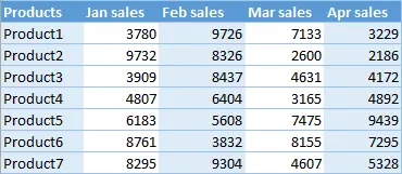
The fastest and easiest way to customize row colors in Excel is to use predefined table styles. Along with other benefits (such as an automatic filter), color alternation is also applied to table rows. To convert a range of data to a table:
- Select the range of cells in which you want to adjust the alternation of row colors.
- On the Advanced tab Insert (Insert) click Table (Table) or click Ctrl + T.
- Ready! Even and odd rows of the created table are colored in different colors. And, what’s great, the automatic color rotation will be preserved when sorting, deleting or adding new rows to the table.

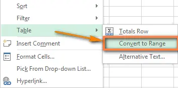
If all the advantages of the table are not needed, and it is enough to leave only the alternating row coloring, then the table is easily converted back to a normal range. To do this, right-click on any cell in the table and in the context menu, click Table > Convert to range (Table > Convert to Range).
Note: If you decide to convert the table to a range, then when new rows are added to the range, the color alternation will not change automatically. There is one more drawback: when sorting data, i.e. when moving cells or rows within the selected range, the color bars will move with the cells, and the neat striped coloring will be completely shuffled.
As you can see, converting a range to a table is a very simple and fast way to highlight alternating rows in Excel. But what if you want a little more?
How to choose your own colors for stripes
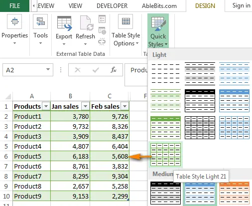
If the standard blue and white palette of an Excel spreadsheet does not excite you, then there are many templates and colors to choose from. Just select the table, or any cell of this table, and then on the tab Constructor (Design) in the section Table styles (Table Styles) choose the appropriate color.
You can scroll through the collection of styles using the arrows or click on the button More options (More) to show all styles. When you hover your mouse pointer over any style, it is immediately applied to the table, and you can immediately see how the alternating rows will look like.
How to highlight different number of rows in table bands
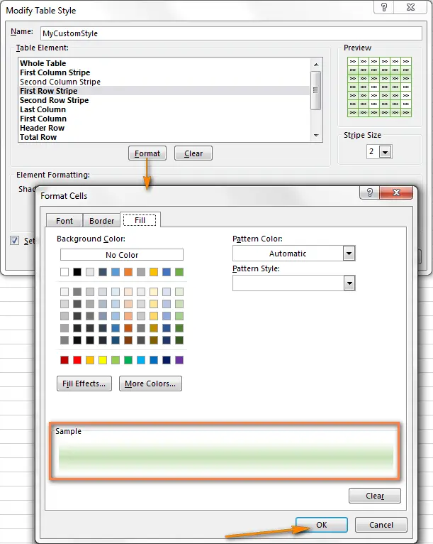
If in each of the colored bars you need to highlight a different number of rows of an Excel sheet, for example, color two rows with one color and the next three with a different color, then you need to create a custom table style. Let’s assume that we have already converted the range to a table and follow the steps below:
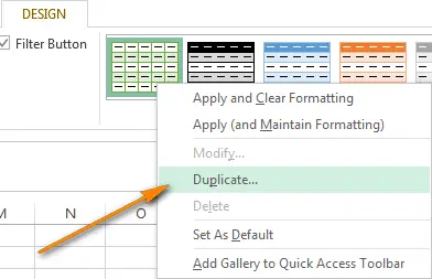
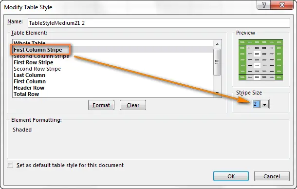
- Let’s open a tab Constructor (Design), right-click on the table style you like and in the menu that appears, click Duplicate (Duplicate).
- In the First name (Name) enter a suitable name for the new table style.
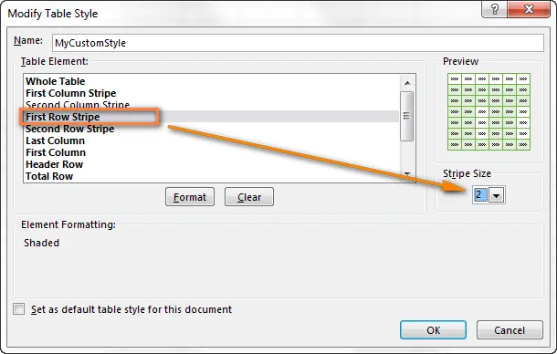
- Let’s select an element First line of lines (First Row Stripe) and establish Strip size (Stripe Size) equal to 2 or another value (optional).
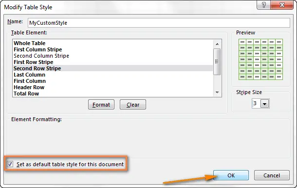
- Next, select an element Second strip of lines (Second Row Stripe) and repeat the process.
- We press OKto save the custom style.
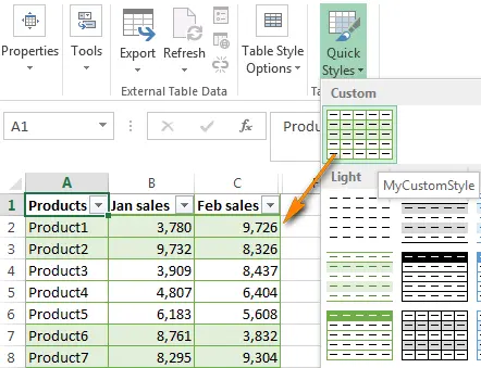
- Select the newly created style in the gallery Table styles (Table Styles). The created styles are at the top of the gallery in the section Custom (Custom).
Note: Custom table styles are only stored in the current workbook, i.e. they will not be available in other books. To use a custom style as the default for all created tables in the current workbook when creating or changing a style in the dialog box Changing the style of a table (Modify Table Style) check the box Set as the default table style for this document (Set as default table style for this document).
If the created style turned out not quite the way you wanted, you can easily change it. To do this, open the styles gallery, find our custom style, right-click on it and select from the context menu Change (Modify). This is where you need to unleash your creative thinking! We press the button Framework (Format) as shown in the figure below, and on the tabs Font (Font), Border (border) and Fill (Fill) of the dialog box that opens, any settings of the corresponding parameters are available to us. You can even set up gradient fills for alternating rows.
Remove line coloring stripe in Excel in one click
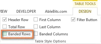
If you no longer need color alternation in an Excel spreadsheet, you can literally remove it with one click. Select any table cell, open the tab Constructor (Design) and uncheck the option line Interleaved lines (Banded rows).
As you can see, the standard table styles in Excel give you a lot of opportunities to create alternating coloring of rows on a sheet and allow you to customize your own styles. I am sure they will help out in many situations. If you want something special, for example, to customize the coloring of the entire row, depending on the change in the selected value, then in this case you need to use conditional formatting.
Alternate line colors with conditional formatting
It is clear without further ado that setting up conditional formatting is a slightly more complex process than applying Excel table styles just discussed. Conditional formatting has one absolute plus – complete freedom for creativity, the ability to color the table in multi-colored stripes exactly as it is needed in each individual case. Later in this article, we will look at several examples of formulas for alternating row coloring in Excel:
Highlight every second row in Excel using conditional formatting
Let’s start with a very simple formula with the function THE REST (MOD) that highlights every second row in Excel. In fact, the same result can be achieved with Excel table styles, but the advantage of conditional formatting is that it works with both tables and simple ranges of data. And this means that when sorting, adding or deleting lines in a range, the coloring is not mixed.
Let’s create a conditional formatting rule like this:
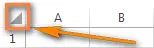
- Select the cells for which you want to change the color. If you need to color the lines on the entire sheet, then click on the gray triangle in the upper left corner of the sheet – so the sheet will be completely selected.
- On the Advanced tab Home (Home) section Styles (Styles) click Conditional Formatting (Conditional Formatting) and in the menu that opens, select Create Rule (New Rule).
- In the dialog box Sozgiving a formatting rule (New Formatting Rule) select an option Use a formula to determine which cells to format (Use formula to determine which cells to format) and enter the following formula:
=ОСТАТ(СТРОКА();2)=0=MOD(ROW(),2)=0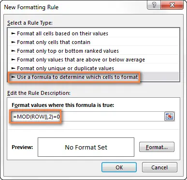
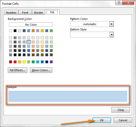
- Then press the button Framework (Format), in the dialog box that opens, select the tab Fill (Fill) and select a fill color for the interleaved lines. The selected color will be shown in the box. Sample (sample). If everything suits – click OK.
- In the dialog box Create a formatting rule (New Formatting Rule) click again OK, and the created rule will be applied to every second row in the selected range.
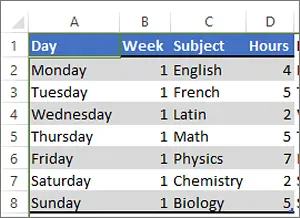
Here’s what I got in Excel 2013:
If instead of alternating with white lines, you want to color the lines in two different colors, then create another conditional formatting rule with the following formula:
=ОСТАТ(СТРОКА();2)=1
=MOD(ROW(),2)=1
Now even and odd lines are highlighted in different colors:

Simple, right? Now I want to briefly explain the syntax of the function THE REST (MOD) as we will be using it in slightly more complex examples later on.
Function THE REST (MOD) – Returns the remainder of a division and has the following syntax:
ОСТАТ(число;делитель)
For example, the result of calculating the formula
=ОСТАТ(4;2)
=MOD(4,2)
will be 0, because 4 is divisible by 2 without a remainder.
Now let’s take a closer look at what exactly the function we created in the previous example does. THE REST (MOD). We used the following combination of functions THE REST (MOD) and LINE (ROW):
=ОСТАТ(СТРОКА();2)
=MOD(ROW(),2)
The syntax is simple and unsophisticated: the function LINE (ROW) returns the row number, then the function THE REST (MOD) divides it by 2 and returns the remainder of the division. When applied to our table, the formula returns the following results:
| Term No | Formula | Result |
|---|---|---|
| Line 2 | =ОСТАТ(2;2) | 0 |
| Line 3 | =ОСТАТ(3;2) | 1 |
| Line 4 | =ОСТАТ(4;2) | 0 |
| Line 5 | =ОСТАТ(5;2) | 1 |
Did you see a pattern? For even rows, the result is always 0, and for the odd ones 1. Next, we create a conditional formatting rule that tells Excel to color odd rows (result is 1) one color and even rows (result 0) a different color.
Now that we’ve got the basics out of the way, let’s move on to more complex examples.
How to set up alternating row groups of different colors
The following formulas can be used to colorize a given number of lines, regardless of their content:
- Coloring odd groups of rows, that is, highlight the first group with color and then through one:
=ОСТАТ(СТРОКА()-НомерСтроки;N*2)+1N=MOD(ROW()-НомерСтроки,N*2)+1N - Coloring Even Groups of Rows, that is, the second and then through one:
=ОСТАТ(СТРОКА()-НомерСтроки;N*2)>=N=MOD(ROW()-НомерСтроки,N*2)>=N
Here Line Number is the row number of the first cell with data, and N is the number of rows in each colored group.
Tip: If you want to highlight both even and odd row groups, then you have to create two conditional formatting rules for each of the above formulas.
The following table shows some examples of using formulas and the formatting result.
| Color every 2 lines, starting with group 1. The data starts on line 2. | =ОСТАТ(СТРОКА()-2;4)+1 | 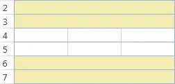 |
| Color every 2 lines starting from group 2. The data starts on line 2. | =ОСТАТ(СТРОКА()-2;4)>=2 | 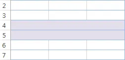 |
| Color every 3 lines starting from group 2. The data starts on line 3. | =ОСТАТ(СТРОКА()-3;6)>=3 | 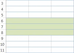 |
How to color strings with three different colors
If you decide that the data will look better if it is colored in three different colors, then create three conditional formatting rules with the following formulas:
- To select the 1st, 4th, 7th and so on lines:
=ОСТАТ(СТРОКА($A2)+3-1;3)=1=MOD(ROW($A2)+3-1,3)=1 - To select the 2st, 5th, 8th and so on lines:
=ОСТАТ(СТРОКА($A2)+3-1;3)=2=MOD(ROW($A2)+3-1,3)=2 - To select the 3rd, 6th, 9th and so on lines:
=ОСТАТ(СТРОКА($A2)+3-1;3)=2=MOD(ROW($A2)+3-1,3)=0
In this example, rows are relative to the cell A2 (i.e. relative to the second row of the Excel sheet). Don't forget instead A2 substitute a link to the first cell of your data.
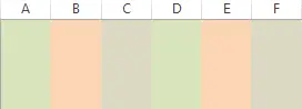
The coloring of the resulting table should look something like this:
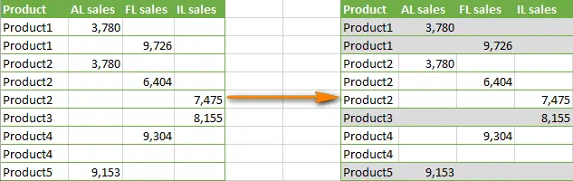
How to change row colors based on the value they contain
This task is similar to the previous one, where we changed the color for a group of rows. The difference is that the number of rows in each group can be different. I'm sure it will be easier to understand with an example.
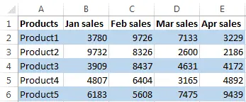
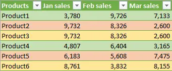
Suppose we have a table that collects data from various sources, such as sales reports from various regions. We want to colorize the first group of rows for the first product (Product 1) with one color, the group of rows for the second product (Product 2) with the second color, and so on. Column A, which contains a list of products, we can use as a key column or a column with unique identifiers.
To set up row color alternation based on the value they contain, we need a slightly more complex formula and an auxiliary column:
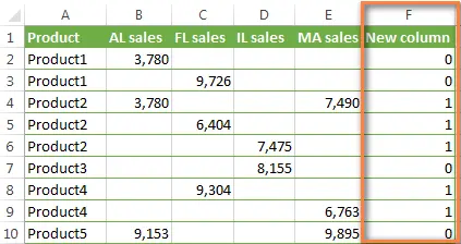
- On the right side of the table, add an auxiliary column, in our example it will be a column F. We can hide it later.
- To cell F2 enter the following formula (assuming row 2 is the first row of data) and then copy it to all the cells in the column:
=ОСТАТ(ЕСЛИ(СТРОКА()=2;0;ЕСЛИ(A2=A1;F1;F1+1));2)=MOD(IF(ROW()=2,0,IF(A2=A1,F1,F1+1)),2)The formula will fill the column F a sequence of groups of 0's and 1's, with each new group beginning on the line in which the new product name appears.
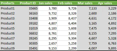
- And finally, we create a conditional formatting rule with the formula:
=$F=1If you want two colors to alternate in the table instead of the color and white stripes, as shown in the figure below, you can create another rule:
=$F=0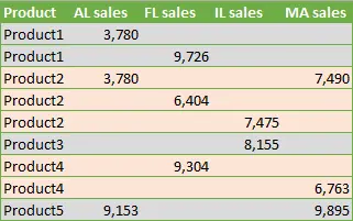
Alternating Column Colors in Excel (Alternating Columns)
In fact, coloring columns in Excel is very similar to striping rows. If all the material of the article read up to this point does not cause difficulties, then you will cope with this topic effortlessly 🙂
The two main ways to color columns in Excel are:
Alternate column colors in Excel using table styles
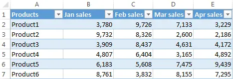
- First of all, let's convert the range to a table (Ctrl+T).
- Then on the tab Constructor (Design) uncheck the line Interleaved lines (Banded rows) and tick the row Striped columns (Banded columns).

- Voila! Columns are colored with standard table colors.
If you want prettier colors, any template from the table style gallery is at your service.
If you want to color a different number of columns with each color, then copy and customize the selected existing table style, as described earlier. In this case, the dialog box Changing the style of a table (Modify Table Style) instead First line of lines (First Row Stripe) и Second strip of lines (Second Row Stripe) need to be selected accordingly First bar of columns (First Colum Stripe) и Second bar of columns (Second Colum Stripe).
This is how an arbitrary column color setting can look like in Excel:
Alternating column colors with conditional formatting
The formulas for setting up alternate column colors in Excel are very similar to the formulas we previously used for row color alternation. The difference is that in combination with the function THE REST (MOD) instead of a function LINE (COLUMN) you need to use the function COLUMN (COLUMN). I will show some examples of formulas in the table below. I have no doubt that you yourself can easily convert formulas for rows into formulas for columns by analogy:
| For coloring every second column | =ОСТАТ(СТОЛБЕЦ();2)=0 | 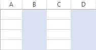 |
| For alternating coloring of groups of 2 columns, starting with the 1st group | =ОСТАТ(СТОЛБЕЦ()-1;4)+1 | 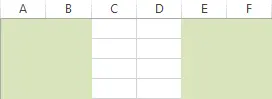 |
| To color columns with three different colors | =ОСТАТ(СТОЛБЕЦ()+3;3)=1
|  |
I hope that now setting the alternating coloring of rows and columns in Excel will not cause difficulties, and you will be able to make the worksheet more attractive, and the data on it more understandable. If you need to customize the alternating coloring of rows or columns in some other way, feel free to write to me, and together we will solve any problem. Thank you for your attention!