


This section of the tutorial provides step-by-step instructions on how to create an advanced pivot table in modern versions of Excel (2007 and newer). For those who work in earlier versions of Excel, we recommend the article: How to create an advanced pivot table in Excel 2003?
We use the company’s first quarter 2016 sales data table as input for building the pivot table.
| A | B | C | D | E | |
|---|---|---|---|---|---|
| 1 | Date | Invoice Ref | Amount | Sales Rep. | Region |
| 2 | 01/01/2016 | 2016 – 0001 | $ 819 | Barnes | North |
| 3 | 01/01/2016 | 2016 – 0002 | $ 456 | Brown | South |
| 4 | 01/01/2016 | 2016 – 0003 | $ 538 | Jones | South |
| 5 | 01/01/2016 | 2016 – 0004 | $ 1,009 | Barnes | North |
| 6 | 01/02/2016 | 2016 – 0005 | $ 486 | Jones | South |
| 7 | 01/02/2016 | 2016 – 0006 | $ 948 | Smith | North |
| 8 | 01/02/2016 | 2016 – 0007 | $ 740 | Barnes | North |
| 9 | 01/03/2016 | 2016 – 0008 | $ 543 | Smith | North |
| 10 | 01/03/2016 | 2016 – 0009 | $ 820 | Brown | South |
| 11 | … | … | … | … | … |
In the following example, we will create a PivotTable that shows monthly sales totals for the year, broken down by region and salesperson. The process of creating this pivot table is described below.
- Select any cell in the range, or the entire range of data that you want to use to build the PivotTable.COMMENT: If you select one cell in a data range, Excel will automatically determine the range for creating a pivot table and expand the selection. In order for Excel to select a range correctly, the following conditions must be met:
- Each column in the data range must have a unique header.
- The data range must not contain empty lines.
- Click on the button summary table (Pivot Table) in section Tables (Table) tab Insert (Insert) Excel menu ribbons.
- A dialog box will open Create a PivotTable (Create PivotTable) as shown in the figure below.

 Make sure that the selected range covers exactly those cells that should be used to create a pivot table. Here you can also choose where the created pivot table should be placed. You can add a pivot table To an existing sheet (Existing Worksheet) или To a new sheet (New Worksheet). Click OK.
 - An empty pivot table and panel will appear Pivot table fields (Pivot Table Field List), which already contains several data fields. Note that these fields are headers from the source data table. We want the PivotTable to show monthly sales totals broken down by region and by salesperson. To do this, in the panel Pivot table fields (Pivot Table Field List) do this:
- Drag box Date to the area Rows (Row Labels);
- Drag box Amount to the area Σ Values (Σ Values);
- Drag box Region to the area Колонны (Column Labels);
- Drag box Sales Rep. to the area Колонны (Column Labels).

- As a result, the pivot table will be filled with daily sales values for each region and for each seller, as shown below.
 To group data by month:
- Right-click on any date in the leftmost column of the pivot table;
- In the context menu that appears, click Group (Group);
- A dialog box will appear Grouping (Grouping) for dates (as shown in the figure below). In field With a step (By) select Months (Months). By the way, you can also group dates and times by other time periods, for example, by quarters, days, hours, and so on;
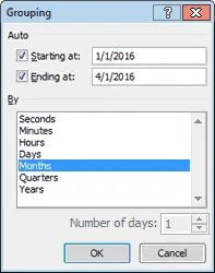
- Press OK.
As required, our PivotTable (see image below) now shows sales totals by month, broken down by region and by salesperson.

To improve the appearance of the PivotTable, you should adjust the formatting. For example, if for the values in the columns B – G set up the currency format, then it will become much easier to read the pivot table.
Filters in a PivotTable
Filters in a PivotTable allow you to display information for a single value or selectively for multiple values from the available data fields. For example, in the pivot table shown above, we will only be able to view data for the sales region North or only for the region South.
To display data for a sales region only North, in panels Pivot table fields (Pivot Table Field List) drag the field Region to the area filters (Report Filters).

Field Region will appear at the top of the pivot table. Open the drop-down list in this field and select the region in it North. The pivot table (as shown in the image below) will only show the values for the region North.

You can quickly switch to viewing region-only data South – for this you need in the drop-down list in the field Region select South.