Advanced filter in Excel

In the last lesson, we met and learned how to apply standard filtering in Excel. But very often situations arise when the basic filtering tools are powerless and cannot provide the required sampling result. In this tutorial, you will learn how to solve this problem in Excel using advanced filters.

If suddenly there is a need to highlight some specific data, then, as a rule, the basic filtering tools can no longer cope with this task. Luckily, Excel comes with many advanced filters, including text search, date search, and numeric filtering, to narrow down your results and help you find exactly what you’re looking for.

Filtering and searching in Excel

Excel allows you to search for information that contains an exact phrase, number, date, and more. In the following example, we will use this tool to leave only brand products in the equipment log. Saris.

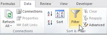
1. Click the Data, then press command Filter. An arrow button appears in each column heading. If you have already applied filters in the table, you can skip this step.
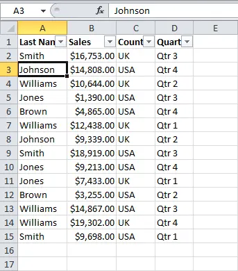
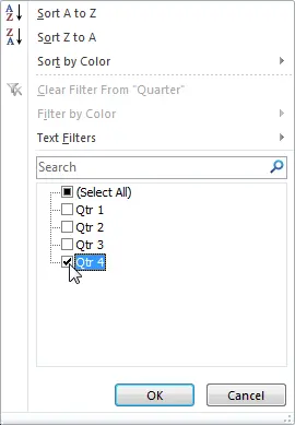
2. Click the arrow button in the column you want to filter. In this example, we will select column C.
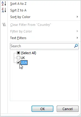
3. The filter menu will appear. Enter a keyword in the search bar. The search results will appear below the field automatically after entering the keyword. In our example, we will enter the word “saris” to find all equipment of this brand.
4. After completing all the steps, click OK.
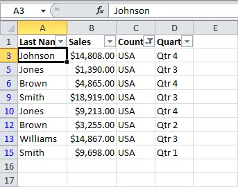
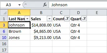
5. The data in the sheet will be filtered according to the keyword. In our example, after filtering, the table contains only equipment of the brand Saris.

Using advanced text filters in Excel

Advanced text filters are used to display more specific information, such as cells that do not contain a given character set. Let’s say our table is already filtered in such a way that in the column A type displayed only Others products. In addition, we will exclude all positions containing the word “case” in the column Equipment description.

1. Click the Data, then press command Filter. An arrow button appears in each column heading. If you have already applied filters in the table, you can skip this step.
2. Click the arrow button in the column you want to filter. In our example, we will select column C.
3. The filter menu will appear. Move the mouse pointer over the item Text filters, then select the desired text filter from the drop-down menu. In this case, we will choose does not containto see data that does not contain the specified word.
4. In the dialog box that appears Custom AutoFilter enter the desired text in the field to the right of the filter, then click OK. In this example, we will enter the word “case” to exclude all positions containing this word.
5. The data will be filtered by the specified text filter. In our case, only positions from the category are reflected. Others, which do not contain the word “case”.

Use advanced date filters in Excel

Advanced filters by date allow you to highlight information for a specific period of time, for example, for the last year, this month, or between two dates. In the following example, we’ll use an advanced date filter to see equipment that was submitted for inspection today.

1. Click the Data and press command Filter. An arrow button appears in each column heading. If you have already applied filters in the table, you can skip this step.
2. Click the arrow button in the column you want to filter. In this example, we will select column D to see the dates we want.
3. The filter menu will appear. Move the mouse pointer over the item Date filters, then select the desired filter from the drop-down menu. In our example, we will select the item Todayto see the equipment that was tested today.
4. The data will be filtered by the specified date. In our case, we will see only the items of equipment that were submitted for verification today.

Using Advanced Number Filters in Excel

Advanced numeric filters allow you to manipulate data in a variety of ways. In the following example, we will only select equipment that is within the given range of identification numbers.

1. Click the Data, then press command Filter. An arrow button appears in each column heading. If you have already applied filters in the table, you can skip this step.
2. Click the arrow button in the column you want to filter. In this example, we will select column A to see the given row of ID numbers.
3. The filter menu will appear. Move the mouse pointer over the item Numeric filters, then select the desired number filter from the drop-down menu. In this example, we will choose междуto see ID numbers in a specific range.
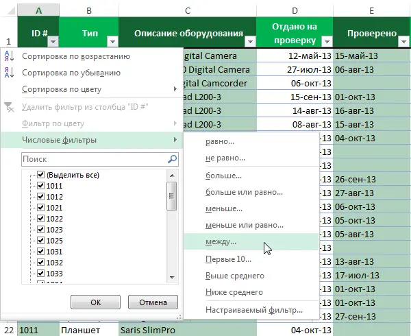
4. In the dialog box that appears Custom AutoFilter enter the required numbers for each of the conditions, then click OK. In this example, we want to get numbers that are greater than or equal to 3000 but less than or equal to 4000.
5. The data will be filtered by the specified numeric filter. In our case, only numbers in the range from 3000 to 4000 are displayed.