


Contents
Yesterday in the marathon 30 Excel functions in 30 days we did simple things with a function T (T). It checks the value to see if it’s text or not, and there are other functions that can do the same thing.
On the 15th day of the marathon, we will devote the study of the function REPT (REPEAT) that repeats a text string a specified number of times. This is another function from the text category, and it has a few interesting points.
Let’s take a closer look at the information and examples by function REPT (REPEAT). If you have additional information and examples on this function, share them in the comments.
Function 15: REPT
Function REPT (REPEAT) repeats a text string a specified number of times. Function REPT (REPEAT) repeats a text string a specified number of times. Function REPT (REPEAT) repeats a text string a specified number of times.
Creating fun effects like the one in the previous paragraph will be much easier thanks to the function REPT (REPEAT). 🙂
How can I use the REPT function?
Function REPT (REPEAT) can be used to fill a cell with a character, as well as in innovative applications such as:
- Create a process indicator or scatter chart inside a cell.
- Keeping a simple count.
- Finding the last text value in a column.
Syntax REPT (REPEAT)
Function REPT (REPEAT) has the following syntax:
REPT(text,number_times)
ПОВТОР(текст;число_повторений)
- text (text) – the text to be repeated.
- numberr_times (number_repeats) is a positive number.
Traps REPT (REPEAT)
- The length of a text string is limited to 32767 characters. If there is more, the formula will report an error.
- If number_times (number_of_repetitions) will be a fraction, it will be truncated to an integer.
- If number_times (number_repeats) will be 0, the result will be an empty string.
Alternatives to REPT (REPEAT)
If you just need to fill a cell with a character, just use cell formatting:
- In a cell, enter the character(s) you want to fill it with, such as a hyphen (-) or a tilde (~).
- Select this cell and click Ctrl + 1to open the window Format Cells (cell format).
- Go to the tab Alignment (Alignment) and in the drop down list Horizontal (horizontal) select Fill (With filling).
- Press OKto close the dialog box.
The symbol will fill the cell. If you expand or narrow the boundaries of the column, then the filling of the cell will follow the change in its size.
Example 1: Progress bar inside a cell
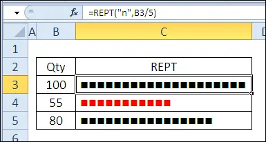
If you do not have one of the latest versions of Excel installed with built-in progress bars, you can create a simple progress bar inside a cell using the function REPT (REPEAT). For example, to create a progress bar for a target value of 100:
- In cell B3, enter 100.
- In cell C3, this formula:
=REPT("n",B3/5)=ПОВТОР("n";B3/5) - For cell C3, set the font Wingdings (font size 9).
- Set the appropriate cell width so that the indicator can fit completely.
- Now changing the number in cell B3 will change the indicator we created.
This example adds conditional formatting to highlight red number less than 60.
Example 2: Scatter plot inside a cell
In addition to progress bars, you can create a simple scatter plot within a cell using the function REPT (REPEAT). For example, to create a scatter plot for a target value of 100:
- In cell B3, enter 100.
- In cell C3, the following formula:
=REPT(" ",B3/5-1)&"o"=ПОВТОР(" ";B3/5-1)&"o" - Set the appropriate cell width so that the indicator can fit completely.
- Now when you change the number in cell B3, the location of the symbol “o«.
Example 3: Keeping a simple count
If you have lost your Cribbage board or are counting the days until your next vacation, you can use the function REPT (REPEAT) to keep track of earned points or elapsed days.
To make a calculation using the function REPT (REPEAT):
- In cell B3, enter a target value, such as 25.
- In cell C3, the following formula:
=REPT("tttt ",INT(B3/5))&REPT("I",MOD(B3,5))=ПОВТОР("tttt ";ЦЕЛОЕ(B3/5))&ПОВТОР("I";ОСТАТ(B3;5)) - Set the font for the cell to Comic Sans or any other font in which the letter t straight line (eventually found a use for Comic Sans!).
- Set an appropriate width for column C. If the target number is large, you can increase the line height and enable text wrapping.
- Change the number in cell C3 and the count will also change.
As a result, this formula will show one group of characters t for every 5 count units. And if there is a remainder after dividing the quantity by 5, this remainder will be shown at the end of the line as characters I – MOD(B3,5) or MOD(B3;5).
Example 4: Finding the last text value in a list
In conjunction with VLOOKUP (VLOOKUP) You can use the function REPT (REPEAT) to return the last text value in the list. For example, if there are text values in column D, use this formula to find the last one:
=VLOOKUP(REPT("z",255),D:D,1)
=ВПР(ПОВТОР("z";255);D:D;1)
Function REPT (REPEAT) in this formula creates a text string of the last letter of the alphabet (zzzz…), and VLOOKUP (VLOOKUP) cannot find such a row. As a result, in the approximate match search mode, the last text value in the list will be selected.