Contents
Yesterday in the marathon 30 Excel functions in 30 days we had a fasting day with a function N (H) where we found out that it can return a number based on the content type of the cell.
On the 23th day of the marathon, we will devote the study of the function FIND (FIND). It is very similar to the function SEARCH (SEARCH), which we met earlier, but the function FIND (FIND) is case sensitive.
So, let’s see the details and examples by function FIND (FIND). If you have additional information or examples, please share them in the comments.
Function 23: FIND
Function FIND (FIND) finds a text string inside another text string, case sensitive.
How can the FIND function be used?
Function FIND (FIND) can find text within a text string, case sensitive. For example:
- Find the starting position of text in a text string.
- Find exact data on a sheet.
- Find the street name in an address.
FIND Syntax
Function FIND (FIND) has the following syntax:
FIND(find_text,within_text,[start_num])
НАЙТИ(искомый_текст;просматриваемый_текст;[нач_позиция])
- find_text (search_text) is the text you are looking for.
- within_text (lookup_text) – text string within which the search is performed.
- start_num (start_position) – if not specified, the search will start from the first character.
Traps FIND (FIND)
- Function FIND (FIND) will return the position of the first matching string, case sensitive. To search in a case insensitive way, use the function SEARCH (SEARCH), which we already considered earlier as part of the marathon 30 Excel functions in 30 days.
- In argument find_text (search_text) functions FIND (FIND) cannot use wildcards. If you still want to use them, then use the function SEARCH (SEARCH).
Example 1: Finding text in a text string
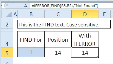
To find the desired text in a text string, use the function FIND (FIND). It is case sensitive, so in the figure below, the first two “i” characters are ignored.
=FIND(B5,B2)
=НАЙТИ(B5;B2)
To handle errors that occur when text is not found, put FIND (FIND) into a function IFERROR (IFERROR). If you have Excel 2003 or earlier, instead of IFERROR (IFERROR) use the function IF (IF) together with ISERROR (EOSHIBKA).
=IFERROR(FIND(B5,B2),"Not Found")
=ЕСЛИОШИБКА(НАЙТИ(B5;B2);"Not Found")

Example 2: Finding Exact Values in a Worksheet
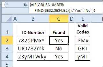
Taking advantage of the fact that the function FIND (FIND) is case sensitive, you can use it to exactly find a string of text within another string. In this example, column E contains Valid Codes. Using the function FIND (FIND) we can determine if the value in cell B2 contains at least one of the valid codes.
This formula must be entered as an array formula by pressing Ctrl + Shift + Enter.
=IF(OR(ISNUMBER(FIND($E$2:$E$4,B2))),"Yes","No")
=ЕСЛИ(ЕЧИСЛО(НАЙТИ($E$2:$E$4;B2)));"Yes";"No")

Example 3: Finding the street name in an address
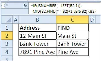
In the following example, most of the addresses in column B start with a number. Using the formula in column C, we check if the first character is a digit. If it is a number, then the function FIND (FIND) finds the first space character, and the function MID (MID) returns all remaining text, starting with the next character.
=IF(ISNUMBER(--LEFT(B2,1)),MID(B2,FIND(" ",B2)+1,LEN(B2)),B2)
=ЕСЛИ(ЕЧИСЛО(--ЛЕВСИМВ(B2;1));ПСТР(B2;НАЙТИ(" ";B2)+1;ДЛСТР(B2));B2)


