


Contents
- 1. Clear the Chart Background
- 2. Move the legend
- 3. Remove the legend if the chart has one data series
- 4. Come up with a meaningful title
- 5. Sort your data before creating a chart
- 6. Don’t make people tilt their heads
- 7. Clean the axles
- 8. Try different themes
- 9. Create a branded chart
- 10. Make the Chart Title Dynamic
We have already talked a lot about how to make data in Excel tables more expressive by setting the cell format and conditional formatting, both for regular tables and for pivot tables. Now let’s do something really fun: let’s start drawing charts in Excel.
In this article, we will not dwell on the basic concepts of plotting. Many examples, if desired, can be found on the Internet or in this section of the site.
1. Clear the Chart Background
When presenting data to an audience, it is very important to get rid of everything that is distracting and focus on what is important. Anyone who has read my Excel articles already knows that I hate grid lines in charts. At first I did not pay attention to them, until I came across several diagrams that made my eyes ripple. This is the problem with unnecessary details: they distract the viewer from what is really important.
Getting rid of grid lines is very easy. First, remember the formatting trick I talk about in each of my articles: to open the format window for anything in Excel (charts or tables), just highlight the item and click Ctrl + 1 – a dialog box for formatting this element will immediately appear.
In our case, you need to select any grid line (except the top one – otherwise the entire construction area will be selected) and call the formatting dialog box. In settings choose Line color > no lines (Line color > No line).
2. Move the legend
I don’t know why Excel places the legend to the right of the chart by default. Most of the time this is very inconvenient. I prefer to move the legend up or down. I like the top better. I only place the legend at the bottom when the top of the chart is already loaded with information, or for a pie chart.
To move the legend, simply open the formatting options (as you just learned how to do!) and under Legend options (Legend Options) select the desired position.
While the legend is selected, change the font size to 12. To do this, you do not need to select the text, just select the legend frame. What looks better – decide for yourself …

3. Remove the legend if the chart has one data series
If the chart shows only one data series, then there is no point in leaving the legend that Excel inserts automatically. It is enough to indicate the name of the series in the title of the chart.
4. Come up with a meaningful title
A common mistake marketers make when creating charts is they forget the title. To the one who collects and processes the data, everything seems absolutely clear. But for those who perceive this information and try to understand what the author means, not everything is so obvious.
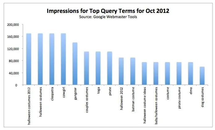
For the diagram shown in the figure below, it would not be enough to write only the word in the title Impressions (impressions) instead Impressions for Top Query Terms for Oct 2012 (Number of impressions for the most popular requests for October 2012).

To add a title to a chart, select it and click Working with charts | Constructor > Chart title (Chart Tools | Layout > Chart Title). I always choose position Above chart (Above Chart).
5. Sort your data before creating a chart
I consider this moment very important. Charts built from unsorted data are much more difficult to read and understand.
If the data is a sequence, such as daily visits for a month or monthly revenue for a year, then chronological sequence is best suited for such data. In other cases, where there is no clear pattern determining the order of elements, the data should be sorted and presented in descending order to show the most significant elements first.
Take a look at the diagram below. I believe you will agree that you need to run your eyes back and forth more than once in order to arrange the shown channels according to the amount of profit.

At the same time, the following diagram is sorted in descending order. As a result, the data is much easier to understand.

Another plus in favor of formatting data as a table before creating a chart from it is the ability to sort. In Excel spreadsheets, sorting is built into the filters provided with headings. If the chart is built on the basis of a table, then it is much easier to change it. For example, as soon as the data in the table is sorted, the chart is automatically updated as well.
6. Don’t make people tilt their heads
Have you ever seen a chart like this one?

Or even worse… like this?
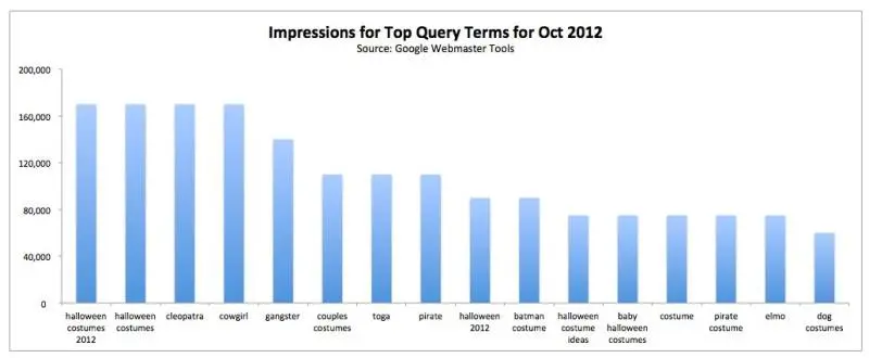
Understanding the data in such a chart is not an easy task, and there is a high risk of making a mistake. If you need to place long labels on the axis, then it is better to expand the plotting area of the chart so that the labels fit horizontally, or even better, use a bar chart instead of a bar chart:

Tip: If you want larger values to be at the top of the graph in a bar chart (as in the chart shown above), then you need to sort the data column in ascending instead of descending order.
In my opinion, this is not entirely logical, but if this is not done, then the most insignificant data will be at the top of the graph. People tend to read charts from top to bottom, so it’s best to put the most important data on top.
7. Clean the axles
Such a diagram resembles a train wreck, in its axes there is everything that I dislike the most.

Before moving on to the axes, let’s remove the grid lines and the legend. Next, we will deal with the five most common errors in the design of the chart axes.
Thousand separators are missing
For values greater than 999, be sure to insert thousands separators. The easiest way is to customize the data formatting in the table. The chart will update automatically.
To add thousands separators, select the entire column and on the tab Home (Home) section Number (Number) click the delimited format button (with three zeros). Excel always adds two decimal places, which you need to get rid of by clicking the decrease decimal place button here, second to the right of the delimited format button.
Another way is to open a dialog Cell format (Format Cells) and customize the formatting in it.
Axle clutter
In the diagram above, the vertical axis is cluttered and overloaded. To tidy it up, select the axis and open the Format Axis dialog box. In chapter Axis parameters (Axis Options) change the parameter Major divisions (Major unit). I changed the value of the major division from 20000 on 40000 – the result is shown in the picture below.
If more graph detail is required, adjust the settings accordingly.

Unnecessary decimals
Never enter decimal places in axis labels, unless 1 (one) is not the maximum value (in other words, except when using fractional numbers for plotting). This mistake is often made when dealing with currencies. Often you can find such signatures: $10, $000.00, $20 and so on. All unnecessary symbols interfere with the perception of the graph.
Decimals instead of percentages
If you need to show percentages on the vertical axis, format them as percentages, do not turn percentages into decimals. The less time a person takes to understand the data, the more compelling it becomes. And again: when working with percentages, discard the fractional part of the number. In other words, don’t leave captions like 10.00%, 20.00%, and so on. Write down just 10%, 20%.
Ridiculous null formatting
Another unpleasant detail is a hyphen instead of zero near the beginning of the vertical axis. This is very common. To learn more about custom number formatting, see the many articles on the topic. There are many interesting formatting possibilities, such as the ability to add text to a number while maintaining the numeric value of the entry.
In our case, we just need to change the zero formatting. To do this, select the column with the source data, open the formatting dialog box and on the tab Number (Number) in the list Number formats (Category) select All formats (Custom). Find the hyphen and replace it with a zero.

As a final touch, I gave the diagram a nicer title, and here is the final result:
8. Try different themes
Excel has quite expressive chart themes, but for some reason most users do not go beyond the standard theme.
Excel 2010 for PC has 53 themes and Excel 2011 for MAC has 57 themes. Each theme comes with its own unique set of designs for 48 chart types. That is, 2544 chart options for PC Excel 2010 and 2736 for MAC Excel 2011.
The theme of the document can be changed by selecting the appropriate one from the drop-down menu on the tab Page layout (Page Layout) in the section Topics (themes). For MAC: Home > Topics (Home > Themes).
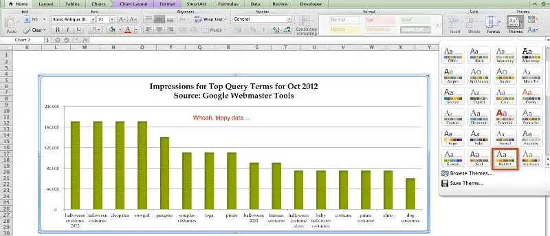
Try different themes, don’t be like everyone else!
9. Create a branded chart
You don’t have to stop at the 2500+ topics offered in Excel. If you want the chart to support corporate style, use corporate colors to create it and then save it as a template.
Suppose you want to develop a marketing plan for a company “Toys R Us”(the author is in no way associated with such a company, if it exists, all coincidences are random), and for the presentation it was decided to build a pie chart using corporate colors. In Excel 2010 (PC) you can use RGB or HSL palettes, in Excel 2011 (MAC) RGB, CMYK or HSB palettes are available.
Since I’m not familiar enough with these palettes, I used the tool Color pickerto define the colors of the company logo “Toys R Us”, and then, using the converter, converted the color encoding to RGB values.
Once you have the desired color values, you can create a chart with any data you want to represent graphically.

Next, you need to select one sector of the pie chart, to do this, click on the diagram once and again on the desired sector. Then change the appearance of this sector using the fill tool on the tab Home (Home) section Font (Font) or in the formatting dialog box.
Suppose we have RGB color codes. Click the drop-down arrow next to the fill tool icon, select More colors and enter the RGB codes in the appropriate fields. Adjust the colors for each chart element in the same way.
As a result, the diagram may turn out, for example, like this:

PC:
To save a diagram as a template on a PC, select it, open the tab Working with charts | Constructor (Chart Tools | Design), click A type > Save Template (Type > Save as Template).
To create a new chart from a template, select the data you want to build a chart on and click Insert (Insert) > Diagrams (Charts) > Other charts (Other Charts) > All diagrams (All Chart Types) > Patterns (Templates) and select the desired template.
Mac:
Right click anywhere in the diagram and select Save as template (Save as Template). The template diagram will be saved in a file .crtx in the chart templates folder.
To create a new chart from a template, select the data you want to build a chart on and click Diagrams (Charts) > Insert Chart (Insert Chart) > Others (Other) > Patterns (Templates) and select the desired template.
10. Make the Chart Title Dynamic
Did you know that you can make a chart title updateable by anchoring it to a worksheet cell? You’ll have to be a little smarter, but such a cool trick will make the boss (or client) look at you like a genius.
Dynamic titles are very useful when the data is regularly updated. This can be, for example, daily numbering, which is entered manually or pulled from some database.
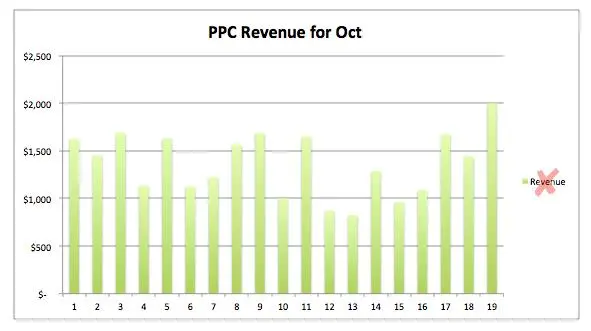
I want to show the company’s income statement “PPCwhich is updated every day. The header will show the total amount for the month to date. Here is how it can be done step by step:
Step 1:
Check that the data is set to the correct number format and that it is formatted as a table, which is essentially a simple database in Excel. You need to format the data as a table because the chart created from the table will update automatically when new rows are added.
In addition, the size of the table is automatically increased by appending new data entered in the bottom row or column to the right of the table.
Step 2:
In a cell below row 31 of the table (to fit a whole month), enter the function SUM (SUM) that sums all the rows in the table – even if some of them are currently empty.

Step 3:
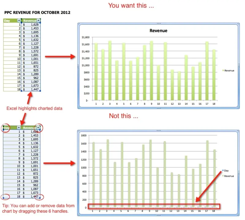
If both columns of our table are used to create data series, then it is enough to select any cell of the table and on the tab Insert (Insert) press Diagrams > bar chart (Charts > Column).
We will select only the header and cells of the column containing profit data. And we will do this because we do not want to create another series of data from the days of the month. To customize the design of the diagram, we have at our disposal a large selection of styles in the section Chart styles (Chart Styles) tab Working with charts | Constructor (Chart Tools | Design).
Step 4:
Add a title to the chart to indicate that there is a running total. I named the diagram: October PPC profit. For more information on adding a title to a chart, see Tip 4 earlier in this article.
Step 5:
By default, the charting area uses a white fill, and as a rule, the chart is shown on a white sheet (and I recommend doing so). We will remove the fill altogether, and this will be a wise move.
To do this, select the chart and click Ctrl + 1then select Fill > No fill (Fill > No Fill). Finally, you need to turn off the grid lines, however, this should be done in any case. This setting is on the tab. View (View) section Show (Show).
Step 6:
Select the cell above the graph to the right of the chart name and create a link in this cell to the cell with the sum. To do this, you just need to enter an equal sign (=) and then click on the cell with the amount or enter the address of this cell manually. Excel highlights the referenced cell with a blue border. Then set the formatting for this cell to be the same as for the chart title.

Step 7:
It remains only to move the chart up so as to align the title with the cell in which the sum is located. It takes a little dexterity to align everything perfectly. Next, we’ll remove the legend because the chart only shows one data series. All is ready! The name has become dynamic.

Step 8:
Now, if you add a new row with data to the table, the chart will dynamically update along with the title. Clever, right?

Translator’s Note: I think many will agree that there is a much easier way to make the chart title dynamic. However, the trick given in this article can also be useful in some situations.
Of course, the chart provides insights that are difficult to achieve by looking at the data in a table. Master the techniques shown in this article and use them in any combination to make your data more compelling in minutes.