How to multiply column by row in excel spreadsheet

When working with Excel spreadsheets, sometimes it becomes necessary to distribute information from one column over several marked rows. In order not to do this manually, you can use the built-in tools of the program itself. The same applies to the reproduction of functions, formulas. When they are automatically multiplied by the required number of lines, you can quickly get the exact result of the calculation.

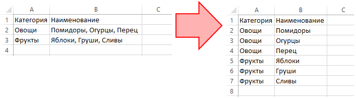
Distribution of data from one column into separate rows

In Excel, there is a separate command with which you can distribute information collected in one column into separate lines.

In order to distribute data, you need to follow a few simple steps:

1. Go to the “EXCEL” tab, which is located on the main page of the tools.
2. Find the block with the “Table” tools, click on it with the left mouse button.
3. From the menu that opens, select the “Duplicate column by rows” option.
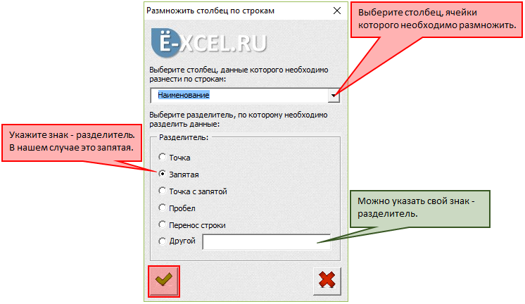
4. After that, a window with the settings for the selected action should open. In the first free field, you need to select from the proposed list the column that you want to multiply.
5. When the column is selected, you need to decide on the type of separator. It can be a dot, comma, semicolon, space, text wrapping to another line. Optionally, you can choose your own character to split.

After completing all the steps described above, a new worksheet will be created on which a new table will be built from many rows in which data from the selected column will be distributed.

Important! Sometimes there are situations when the action of multiplying columns from the main worksheet needs to be noted. In this case, you can undo the action through the key combination “CTRL + Z” or click on the undo icon above the main toolbar.

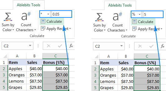
Reproduction of formulas

More often when working in Excel there are situations when it is necessary to multiply one formula at once into several columns in order to obtain the required result in adjacent cells. You can do it manually. However, this method will take too much time. There are two ways to automate the process. With the mouse:

1. Select the topmost cell from the table where the formula is located (using LMB).
2. Move the cursor to the far right corner of the cell to display a black cross.
3. Click LMB on the icon that appears, drag the mouse down to the required number of cells.

After that, in the selected cells, the results will appear according to the formula set for the first cell.

Important! Reproduction of a formula or a certain function throughout the column with the mouse is possible only if all the cells below are filled. If one of the cells does not have information inside, the calculation will end on it.

If a column consists of hundreds to thousands of cells, and some of them are empty, you can automate the calculation process. To do this, you need to perform several actions:

1. Mark the first cell of the column by pressing LMB.
2. Scroll the wheel to the end of the column on the page.
3. Find the last cell, hold down the “Shift” key, click on this cell.

The required range will be highlighted.

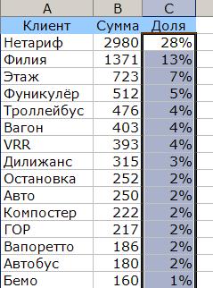
Sort data by columns and rows

Quite often there are situations when, after automatically filling the worksheet with data, they are distributed randomly. To make it convenient for the user to work in the future, it is necessary to sort the data by rows and columns. In this case, as a distributor, you can set the value by font, descending or ascending, by color, alphabetically, or combine these parameters with each other. The process of sorting data using the built-in Excel tools:

1. Right-click anywhere on the worksheet.
2. From the context menu that appears, select the option – “Sort”.
3. Opposite the selected parameter, several options for sorting data will appear.

Another way to select the information sorting option is through the main toolbar. On it you need to find the “Data” tab, under it select the “Sort” item. The process of sorting a table by a single column:

1. First of all, you need to select a range of data from one column.
2. An icon will appear on the taskbar with a selection of options for sorting information. After clicking on it, a list of possible sorting options will open.

If several columns from the page were initially selected, after clicking on the sort icon on the taskbar, a window with the settings for this action will open. From the proposed options, you must select the option “automatically expand the selected range”. If you do not do this, the data in the first column will be sorted, but the overall structure of the table will be broken. Row sorting process:

1. In the sorting settings window, go to the “Parameters” tab.
2. From the window that opens, select the “Range Columns” option.
3. To save the settings, click on the “OK” button.

The parameters that are initially set in the sorting settings do not allow random distribution of data across the worksheet. To do this, you need to use the RAND function.

Conclusion

The procedure for multiplying columns by rows is quite specific, which is why not every user knows how to implement it. However, after reading the instructions above, this can be done very quickly. In addition to this, it is recommended to practice with the reproduction of functions and formulas, due to which it will be possible to save a large amount of time during various calculations in large ranges of cells.