An example of performing a correlation analysis in Excel

One of the most common methods used in statistics to study data is correlation analysis, which can be used to determine the influence of one quantity on another. Let’s see how this analysis can be performed in Excel.

Purpose of correlation analysis

Correlation analysis allows you to find the dependence of one indicator on another, and if it is found, calculate correlation coefficient (degree of relationship), which can take values ​​from -1 to +1:

• if the coefficient is negative, the dependence is inverse, i.e. an increase in one value leads to a decrease in the other and vice versa.
• if the coefficient is positive, the dependence is direct, i.e. an increase in one indicator leads to an increase in the second and vice versa.

The strength of the dependence is determined by the modulus of the correlation coefficient. The larger the value, the stronger the change in one value affects the other. Based on this, with a zero coefficient, it can be argued that there is no relationship.

Performing correlation analysis

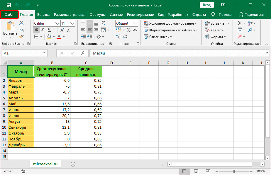
To learn and better understand correlation analysis, let’s try it for the table below.

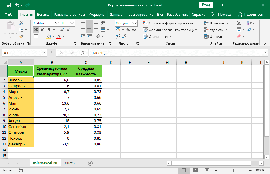
Here are the data on the average daily temperature and average humidity for the months of the year. Our task is to find out if there is a relationship between these parameters and, if so, how strong.

Method 1: Apply the CORREL Function

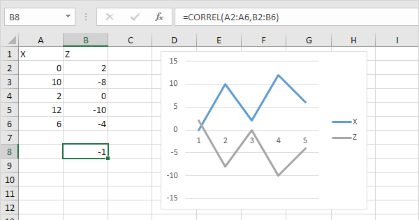
Excel provides a special function that allows you to make a correlation analysis – CORREL. Its syntax looks like this:

КОРРЕЛ(массив1;массив2).

The procedure for working with this tool is as follows:

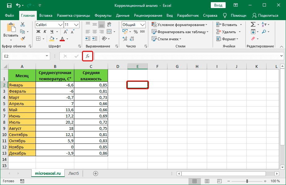
1. We get up in a free cell of the table in which we plan to calculate the correlation coefficient. Then click on the icon “fx (Insert function)” to the left of the formula bar.
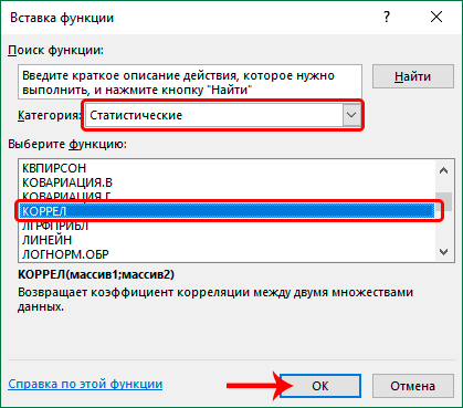
2. In the opened function insertion window, select a category “Statistical” (or “Full alphabetical list”), among the proposed options we note “CORREL” and click OK.
3. The function arguments window will be displayed on the screen with the cursor in the first field opposite “Array 1”. Here we indicate the coordinates of the cells of the first column (without the table header), the data of which needs to be analyzed (in our case, B2: B13). You can do this manually by typing the desired characters using the keyboard. You can also select the required range directly in the table itself by holding down the left mouse button. Then we move on to the second argument “Array 2”, simply by clicking inside the appropriate field or by pressing the key Tab. Here we indicate the coordinates of the range of cells of the second analyzed column (in our table, this is C2: C13). Click when ready OK.
4. We get the correlation coefficient in the cell with the function. Meaning “-0,63” indicates a moderately strong inverse relationship between the analyzed data.

Method 2: Use “Analysis Toolkit”

An alternative way to perform correlation analysis is to use “Package Analysis”, which must first be enabled. For this:

1. Go to the menu “file”.
2. Select an item from the list on the left “Parameters”.
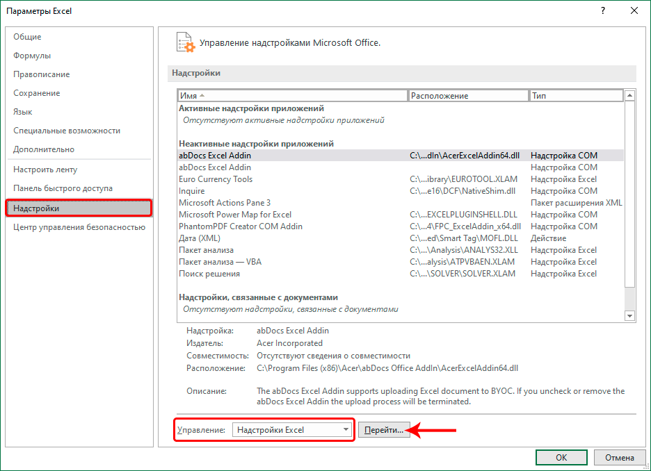
3. In the window that appears, click on the subsection “Add-ons”. Then in the right part of the window at the very bottom for the parameter “Control” Choose “Excel add-ins” and click “Go”.
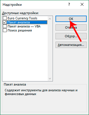
4. In the window that opens, mark “Analysis Package” and confirm the action by pressing the button OK.

All is ready, “Analysis Package” activated. Now we can move on to our main task:

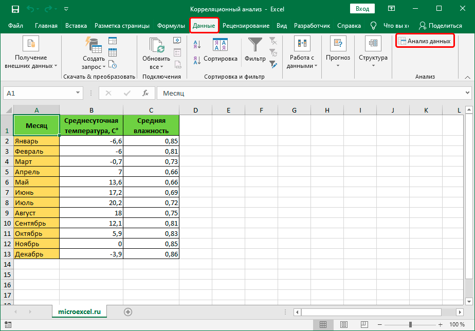
1. Push the button “Data analysis”, which is in the tab “Data”.
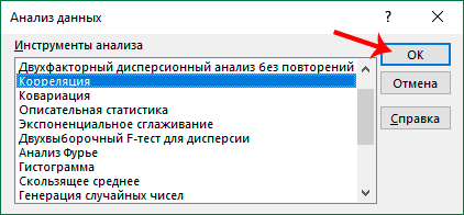
2. A window will appear with a list of available analysis options. We celebrate “Correlation” and click OK.
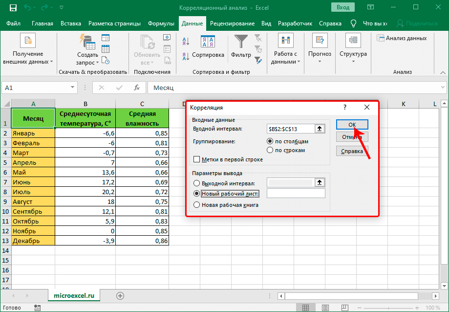
3. A window will appear on the screen in which you must specify the following parameters:
   • “Input Interval”. We select the entire range of analyzed cells (that is, both columns at once, and not one at a time, as was the case in the method described above).
   • “Grouping”. There are two options to choose from: by columns and rows. In our case, the first option is suitable, because. this is how the analyzed data is located in the table. If headings are included in the selected range, check the box next to “Labels in the first line”.
   • “Output Options”. You can choose an option “Exit Interval”, in this case the results of the analysis will be inserted on the current sheet (you will need to specify the address of the cell from which the results will be displayed). It is also proposed to display the results on a new sheet or in a new book (the data will be inserted at the very beginning, i.e. starting from the cell (A1). As an example, we leave “New Worksheet” (selected by default).
   • When everything is ready, click OK.
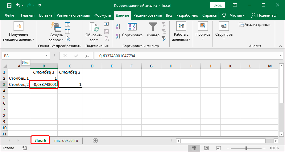
4. We get the same correlation coefficient as in the first method. This suggests that in both cases we did everything right.

Conclusion

Thus, performing correlation analysis in Excel is a fairly automated and easy-to-learn procedure. All you need to know is where to find and how to set up the necessary tool, and in the case of “solution package”, how to activate it, if before that it was not already enabled in the program settings.